Van Leer’s analysis of these methods is a tour-de-force especially considering the sort of resources available to him at that time. He did not have use of tools such as Mathematica upon which I rely. Nonetheless, the modern tools do allow more flexibility in analysis, and exploration of extensions of the methods without undue effort. This is not to say that the analysis is particularly easy as Mathematica analysis goes, it does require considerable skill, experience and attention. My hope for this rearticulation of the results is for clarity with a substantial appreciation for the skill expressed in the original exposition.
Here we briefly review the six schemes presented by Van Leer in that 1977 paper in terms of their basic structure, and numerical properties. We will utilize Von Neumann analysis for both the fully discrete and semi-discrete schemes. In Von Neumann analysis the variable on the mesh is replaced by the Fourier transform,
 or
or 
with  being the angle and
  being the amplification factor.
The fully discrete analysis was the vehicle of presention for Van Leer, and the semi-discrete analysis will be additional detail. The fully discrete schemes all fufill the characteristic condition, they recover the exact solution as the CFL number goes to one, which also demarks its’ stability limit. The semi-discrete analysis only provides the character of the spatial scheme.
Scheme I. The Piecewise Linear Method.
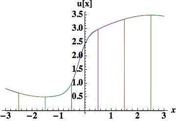
This method uses a piecewise linear reconstruction
 with
with  ,
,  with slopes computed from local data
  .
.
The full update is

with  and
and  is the CFL number.
This method is second-order accurate as verified by expanding the method function in a Taylor series. This can also be verified by expanding the Fourier transformed mesh function in a Taylor series expansion around  .
.

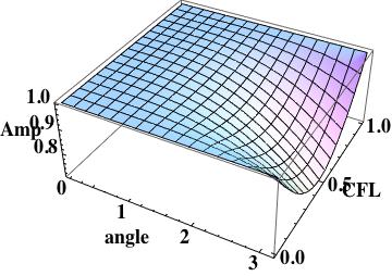
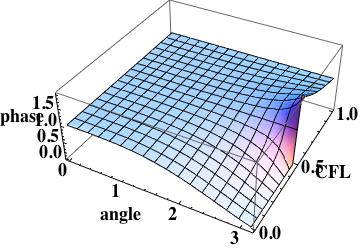
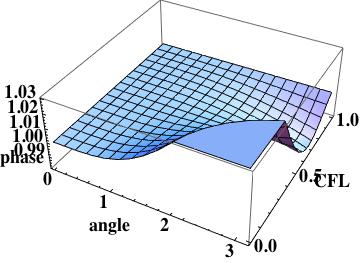
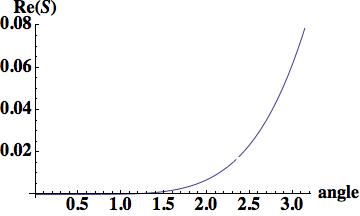
Scheme I amplification surface plot, shows large error at the mesh scale
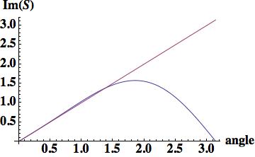
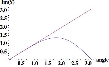
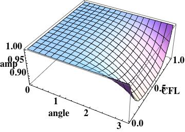
The amplification factor is 
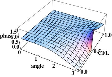
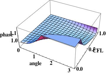
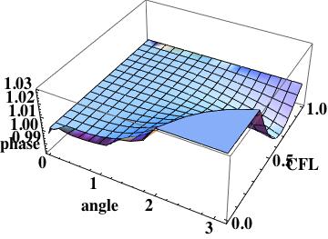
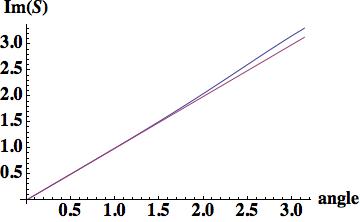
The phase error is  this is the leading order error (being one order higher due to how the phase error is written). A key aspect of this scheme has zero phase error at CFL numbers of one-half and one.

As with the amplification, scheme I has large errors at the mesh scale.
The semi-discrete form is  , which is useful if the scheme is used with a method-of-lines time integration.

Dispersion error for Scheme I is large past 
Scheme II. The Piecewise Linear Method with Evolving Slopes.
This method evolves both the variable and its first derivative and requires the analysis of a system of variables. The scalar analysis of stability is replaced by the analysis of a matrix determined by the behavior of its eigenvalues. One eigenvalue will define the behavior of the scheme, while the second eigenvalue has be referred to as spurious. More recently it has been observed that the “spurious’’ eigenvalue describes the subcell behavior at the mesh scale.
The method uses the same reconstruction as Scheme I, but evolves both and  in time. The update is then two equations, one for the cell-centered data,
 ,
,
which is identical to Scheme I and a second for the slopes
 ,
,
where the usual  as the initial slope is replaced by the first expression on the right hand side of the equation driving a coupling of the variable and the slope in the update.
The slope update is unusual and causes significant error as the CFL number goes to zero. This method does not have an obvious method of lines form due to the nature of this update.
The amplification factor is  .
.

The phase error is  and is the leading order error as with all of the first three methods. Again, this method does not lend itself to a well-defined semi-discrete method.

Scheme III. The Piecewise Linear Method with Evolving First Moment.
This method uses a reconstruction that is similar to piecewise linear, but instead of slope (first derivative), the linear term is proportional to the moment of the solution,
again  , but
, but  . Here, as with Scheme II, we evolve both
  , and
, and  , but the evolution equation for is much different, and naturally yields a coupled system. This also provides a direct path to writing the scheme in a semi-discrete form.
The update for is the same as the previous two schemes,
.
The update for is based on the weak form of the PDE and uses the definition of the first moment,
 ,
, ![\partial_t m - \int_{-1/2}^{1/2} \partial_x \xi u d\xi + [u(1/2)+u(-1/2)] = 0](https://s0.wp.com/latex.php?latex=%5Cpartial_t+m+-+%5Cint_%7B-1%2F2%7D%5E%7B1%2F2%7D+%5Cpartial_x+%5Cxi+u+d%5Cxi+%2B+%5Bu%281%2F2%29%2Bu%28-1%2F2%29%5D+%3D+0&bg=ffffff&fg=000&s=0&c=20201002) .
.
Discretely this equation can be evaluated for the scalar wave equation to
 , where
  .
.
The amplification factor is  .
.

The phase error is  now the amplification error is leading and the method is confirmed as being third-order. This scheme is obviously more accurate than the previous two methods.

The semi-discrete form follows from the standard updates for both the variable and its moment without any problem. The update has an accuracy of second order with small coefficients,  , which the keen observer will notice being third-order accurate instead of the expected second order. Van Leer made a significant note of this.


Scheme IV. The Piecewise Parabolic Method.
This method uses a piecewise parabolic reconstruction
 ,
,
and uses the variables and its two nearest neighbors to determine the fit. The fit is defined as recovering the integral average in all three cells. The coefficients are then simply defined by ,  , and
, and  . This is a third-order method.
The update is simple based on the evaluation of edge and time-centered values that need to be considered slightly differently for third-order methods,
 . The update then is simply the standard conservative variable form,
 .
.
The amplification factor is 

The phase error is  this is the leading order error (being one order higher due to how the phase error is written). A key aspect of this scheme has zero phase error at CFL numbers of one-half and one.

The semi-discrete form is  , which is useful if the scheme is used with a method-of-lines time integration.


Scheme V. The Piecewise Parabolic Edge-Based Method.
This method uses a piecewise parabolic reconstruction
,
and uses the variables and its two edge values determining the fit. The fit recovers the integral of the cell  and the value at the edges
  . The coefficients are then simply defined by ,
  , and
, and  . This is a third-order method.
This method is distinctly different than Scheme IV in that both the cell-centered, conserved quantities, and the edge-centered (non-conserved) quantities. The form of the updates are distinctly different and derived accordingly. The time-integrated edge value follows the polynomial form from Scheme IV,
 ,
,
giving a cell centered update, . The edge update is defined by a time-integrated, upstream-biased first derivative evaluated at the cell-edge position,
 .
.
The amplification factor is .

The phase error is now the amplification error is leading and the method is confirmed as being third-order. The scheme is very close in performance and formal error form to Scheme III, but is arguably simpler.

The semi-discrete form follows from the standard updates for both the variable and its moment without any problem. The update has an accuracy of third order with small coefficients,  .
.


Looking at the recent PPML (piecewise parabolic method – local) scheme of Popov and Norman produces an extremely interesting result. The interpolation used by PPML is identical to Scheme V, but there is a key difference in the update of the edge values. The differential form of evolution is not used and instead a semi-Lagrangian type of backwards characteristic interpolation is utilized,
 .
.
This produces exactly the same scheme as the original Scheme V for the scalar equation. In many respects the semi-Lagrangian update is simpler and potentially more extensible to complex systems. Indeed this may be actualized by the PPML authors who have applied the method to integrating the equations of MHD.
Scheme VI. The Piecewise Parabolic Method with Evolving First and Second Moments.
This method uses a piecewise parabolic reconstruction
,
and uses the variables and its two edge values determining the fit. The fit recovers the integral of the cell and the value at the edges . The coefficients are then simply defined by  ,
,  , and
, and 
 .
.  is the first moment of the solution, and
  is the second moment. The moments are computed by integrating the solution multiplied by the coordinate over the mesh cell. This is a fifth-order method.
For all the power Mathematica provides, this scheme’s detailed analysis has remained elusive, so the results are only presented for the semi-discrete case where Mathematica remained up to the task. Indeed I did get results for the fully discrete scheme, but the plot of the amplification error was suspicious and for that reason will not be shown, nor will the detailed truncation error associated with the Taylor series.
The semi-discrete form follows from the standard updates for both the variable and its moment without any problem. The update has an accuracy of second order with small coefficients,  , which the keen observer will notice being fifth-order accurate instead of the expected third order. The semi-discrete update for the first moment is
  , and the second moment is
 .
.


 .
.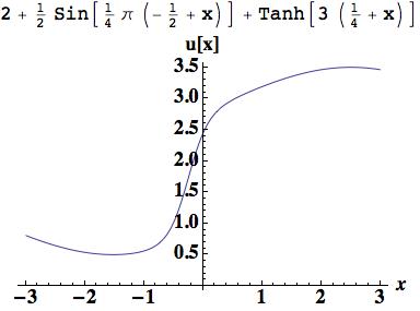
 , which is the foundation of Godunov’s method, a first-order, but monotone method. The integrated difference between the analytical function and this piecewise polynomial is 0.882015, which will serve as a nice measure of success with higher order reconstructions.
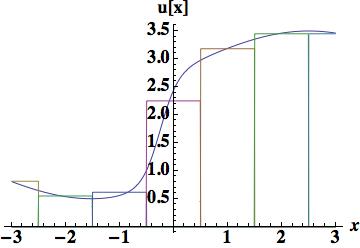
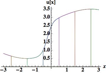
 . The improvement over the piecewise constant is obvious and the integrated error is now, 0.448331 about half the size of the piecewise constant.
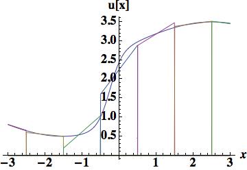
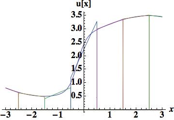
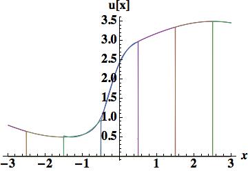
 . We stay with Van Leer’s use of Legendre polynomials because they are mean preserving without difficulty. The first is the parabola determined by the three centered cell center values, which gives a relatively large error of 0.427028 almost as large as the piecewise linear interpolation.

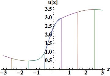
 . We will look at two reconstructions, the first based on three cell-centers, and an integral of the derivative in the center cell. This is a Hermite scheme, and based on previous experience with Schemes 1 and 4 we should expect its performance to be relatively poor with an error of 0.14884, one-third of that found with the piecewise parabolic scheme 4. The second cubic reconstruction will use the cell-center, edges and the first moment, provides excellent results, 0.044014 approximately on par with the two moment piecewise parabola the basis of scheme 6. The method to update the degrees of freedom is arguably simpler (and the overall degrees of freedom is equivalent).
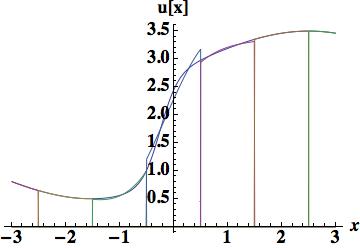
 . Four different methods will be used to determine the coefficients. The first is a fairly important approach because the evaluation provides the stencil used for the upstream-centered fifth order WENO flux. This polynomial is determined by the cell-centered values in the cell and the two cells to the left or right. The figure shows that the polynomial is relatively poor in terms of accuracy, and confirmed by the integrated error, 0.404114 barely better than the parabola used for scheme 4. The quartic reconstruction must provide greater value.
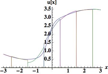

 . Five cell-center values participate in the scheme,
  . The standard approach then derives parabolic approximations based on stencil using cells,
  ,
,  , and
, and  . By some well-defined means the smoothest stencil among the three is chosen to update
  ,
,  , and
, and  . Weights are defined by using the derivatives of the corresponding parabolas to measure the smoothness of each. The weights are chosen so that in smooth regions the weights give a fifth-order approximation to the edge value,
  . The point is that the same principles could be used for other schemes, indeed they already have been in the case of Hermitian WENO methods.
 ,
,  and
and  . This gives a parabola of
 .
. .
. and
and  .
. .
. ,
,  .
. .
. and cell-edge values,
  . This defines a quartic polynomial,


 .
. . This is exceedingly accurate with the dispersion relation peaking at
  with an error of only 2.5%.
 , and the edge-first-derivatives,
  .It is also similar to the PQM method proposed for climate studies. The PQM method is implemented much like PPM in that the edge variables are approximated in terms of the cell-centered degrees of freedom. Here we will describe these variables as independent degrees of freedom. The polynomial reconstruction defined by these conditions is


 .
. . This is exceedingly accurate with the dispersion relation peaking at $latex\theta=\pi$ with an error of only 1.2%.
 .
. .
.

 .
. . This is exceedingly accurate with the dispersion relation peaking at $latex\theta=\pi$ with an error of only 3.1%.

 .
. . This is accurate with the dispersion relation peaking at $latex\theta=\pi$ with an error about 12%.

 .
. . This is accurate with the dispersion relation peaking at $latex\theta=\pi$ with an error of 10%. The last two methods may not be particularly interesting in and of themselves, but may be useful as alternative stencils for ENO-type methods.
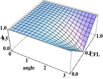


 ,
, , where
  .
.