• About The Regularized Singularity

The Regularized Singularity

~ The Eyes of a citizen; the voice of the silent

The Regularized Singularity

Monthly Archives: July 2014

What is the future of Computational Science, Engineering and Mathematics?

24 Thursday Jul 2014

Posted by Bill Rider in Uncategorized

≈ 2 Comments

I spent the week at a relatively massive conference (3000 attendees) in Barcelona Spain, the World Congress on Computational Mechanics. The meeting was large enough that I was constantly missing talks that I wanted to see because other talks were even more interesting. Originally I wanted to give four talks, but the organizers allowed only one so I was attending more talks and giving far less. Nonetheless such meetingsBarcelona-Photoxpress_8240667 are great opportunities to learn about what is going on around the World, get lots of new ideas, meet old friends and make new ones. It is exactly what I wrote about a few weeks ago, giving a talk is second, third or even fourth on the list of reasons to attend such a meeting.

The span and scope of the Congress is truly impressive. Computational modeling has become a pervasive aspect of modern science and engineering. The array of application is vast and impressively international in flavor. While all of this is impressive, such venues offer an opportunity to take stock of where I am, and where the United States and the rest of the World stand. All of this provides a tremendously valuable opportunity to gain much needed perspective.

An honest assessment is complex. On the one hand, the basic technical and scientific progress is immense, on the other hand there are concerns lurking around every corner. While the United States probably remain in a preeminent state for computational science and engineering, the case against this is getting stronger every day. Europe and Asia are catching up quickly if not having overtaken the USA in many subfields. Across the board there are signs of problems and stagnation in the field. It would seem clear that people know this and it isn’t clear whether there is any action to address problems. Among these issues is the increased use of a narrow set of software tools either commercial or open source computational tools with a requisite lack of knowledge and expertise in the core methods and algorithms used inside them. In addition, the nature of professional education and the state of professionalism is under assault by societal forces,

Evernote Camera Roll 20140723 181749Despite the massive size of the meeting there are substantial signs that support for research in the field is declining in size and changing in character. It was extremely difficult to see “big” things happening in the field. The question is whether this is the sign of a mature field where slow progress is happening, or the broad lack of support for truly game-changing work. It could also be a sign that the creative energy in science has moved to other areas that are “hotter” such biology, medicine, materials, … There was a notable lack of exciting keynote lectures at the meeting. There didn’t seem to be any “buzz” with any of them. This was perhaps the single most disappointing aspect of the conference.

A couple of things are clear in the United States and Europe the research environment is in crisis under assault from short-term thinking, funding shortfalls (after making funding the end-all and be-all), and educational malaise. For example, I was horrified that Europeans are looking to the USA for guidance on improving their education. This comes on top of my increasing concern about the nature of professional development at the sort of Labs where I work, and the general lack of educational vitality at universities. More and more it is clear that the chief measure of academic success for professors in monetary. The claims of research quality are measured in dollars and the publish or perish mentality that has ravaged the scientific literature. It is a system in dire need of focused reform and should not be the blueprint for anything but failure. The monetary drive comes from the lack of support that education is receiving from the government, which has driven tuition higher at a stunning pace. At the same time the monetary objective of research funding is hollowing out the educational focus universities should possess. The research itself has a short-term focus, and the lack of emphasis or priority for developing people be they students or professionals shares the short sighted outcome. We are draining our system of the vital engine of innovation that has been the key to our recent economic successes.

Another clear trend that resonates with my attendance at the SIAM annual meeting a few weeks ago is the increasing divide between applied mathematic (or theoretical mechanics) and applications. The disparity in focus between the theoretically minded scientists and the application-focused scientist-engineer is growing to the detriment of the community. The application side of things is increasingly using commercial codes that tend to reflect a deep stagnation in capability (aside from the user interface). The theoretical side is focused on idealized problems stripped of real features that complicate the results making for lots of results that no one on the applied side cares about or can use. The divide is only growing with fewer and fewer reaching across the chasm to connect theory to application.

The push from applications has in the past spurred the theoretical side to advance by attacking more difficult problems. Those days appear to be gone. I might blame the prevalence of the sort of short-term thinking investing other areas for this. Both sides of this divide seem to be driven to take few chances and place their efforts into the safe and sure category of work. The theoretical side is working on problems where results can surely be produced (with the requisite publications). By the same token the applied side uses tried and true methods to get some results without having to wait or hope for a breakthrough. The result is a deep sense of abandonment of progress on many fronts.

The increasing dominance of a small number of codes either commercial or open source would be another deep concern. Part of the problem is a reality (or perception) of extensive costs associated with the development of software. People choose to use these off-the-shelf systems because they cannot afford to build their own. On the other hand, by making these choices they and their students or staff are denied the hands on knowledge of the methodology that leads to deep expertise. This is all part of this short-term focus that is bleeding the entire community of deep expertise development necessary for excellence. The same attitudes and approach happen at large laboratories that should seemingly not have the sort of financial and time pressures operating in academia. This whole issue is exacerbated by the theoretical versus applied divide. So far we haven’t made scientific and engineering software modular or componentized. Further the leading edge efforts with “modules” often are so divorced from real problems that they can’t really be relied upon for hard-core applications. Again we have problems with adapting to the modern world confounded with the short-term focus, and success measures that do not measure success.

Perhaps what I’m seeing is a veritable mid-life crisis. The field of computational science and engineering has become mature. It is remarkably broad and making inroads into new areas and considered a full partner with traditional activities in most high-tech industries. At the same time there is a stunning lack of self-awareness, and a loss of knowledge and perspective on the history of the past fifty to seventy years that led to this point. Larger societal pressures and trends are pushing the field in directions that are counter-productive and work actively to undermine the potential of the future. All of this is happening at the same time that computer hardware is either undergoing a crisis or phase transition to a different state. Together we are entering an exciting, but dangerous time that will require great wisdom to navigate. I truly fear that the necessary wisdom while available will not be called upon. If we continue to choose the shortsighted path and avoid doing some difficult things, the outcome could be quite damaging.

Evernote Camera Roll 20140723 181903
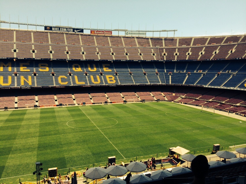
A couple of notes about the venue should be made. Barcelona is a truly beautiful city with wonderful weather, people, architecture food, mass transit, I really enjoyed the visit, and there is plenty to comment on. Too few Americans have visited other countries to put their own country in perspective. After a short time you start to hone in on the differences between where you visit and where you live. Coming from America and hearing about the Spanish economy I expected far more homelessness and obvious poverty. I saw very little of either societal ill during my visit. If this is what economic disaster looks like, then it’s hard to see it as aSanta-Caterina-Market-in-Barcelonan actual disaster. Frankly, the USA looks much worse by comparison with a supposedly recovering economy. There are private security guards everywhere. The amount of security and the meeting was actually a bit distressing. In contrast to this in a week, at a hotel across the street from the hospital, I heard exactly one siren, amazing. As usual getting away from my standard environment is thought provoking, which is always a great thing.

von Neumann Analysis of Finite Difference Methods for First-Order Hyperbolic Equations

21 Monday Jul 2014

Posted by Bill Rider in Uncategorized

≈ 1 Comment

Last week I showed how the accuracy, stability and general properties of an ODE integrator might be studied with the aid of Mathematica. This week I will do the same for a partial differential equations solution. Again, I will provide the commands used in Mathematica to conduct the analysis reported at the end of the post.

It is good to start as simple as possible. That was the reason for retreading the whole ODE stability analysis last week. Now we can steadily go forward toward looking at something a bit harder partial differential equations, starting with a first-order method for a first-order hyperbolic equation, the linear advection equation,

u_t + u_x=0, where the subscript denotes differentiation with respect to the variable. This equation is about as simple as PDEs get, but it is notoriously difficult to solve numerically.

Before getting to the analysis we can state a few properties of the equation. The exact solution is outrageously simple, u \left(x, t \right) = u(x-t,0). This means that the temporal solution is simply defined by the initial condition translated by the velocity (which is one in this case) and time. Nothing changes it simply moves in space. This is a very simple form of space-time self-similarity. If we are solving this equation numerically, any change in the waveform is an error. We can also note that the integral of the value is preserved (of course) making this a “conservation law”. Later when you’d like to solve harder problems this property is exceedingly important.

Now we can proceed to the analysis. The basic process is to replace the function with an analytical representation and similar to ODEs we use the complex exponential (Fourier transform), \exp\left(\imath j \theta\right), where j is the grid index of our discretized function, and \theta is the angle parameterizing frequency of the waveform. The analysis then proceeds much as in the style as the ODE work from last week, one substitutes this function into the numerical scheme and works out the modification of the waveform by the numerical method. We then take this modification to be the symbol of the operator A\left(\theta\right) = \left| A \right\| \exp\left(\imath\alpha\right). In this form we have divided the symbol into two effects its amplitude and its modulation of the waveform or phase. Finishing our conceptual toolbox is the expression of the exact solution as u\left(x,0\right)\exp\left(-\imath t \theta\right) .

We are now ready to apply the analysis technique to the scheme. We can start off with something horribly simple like first-order upwind. The numerical method is easy to write down as u_j^{n+1}=u_j^n-\nu\left(u_{j+1/2}^n-u_{j-1/2}^n\right) where \nu= \Delta t / \Delta x is the Courant or CFL number and u_{j+1/2}^n = u_j^n is the upwind edge value. The CFL number is the similarity variable (dimensionless) of greatest important for numerical schemes for hyperbolic PDEs. Now we plug our Fourier function into the grid values in the scheme and evaluate for a single grid point j=0. Without showing the trivial algebraic steps this gives A = 1 - \nu\left(1-\exp(-\imath \theta)\right). We can make the substitution of the trigonometric functions for the complex exponential, $\exp\left(-\imath \theta\right) = \cos\left(\theta\right) – \imath \sin\left(\theta\right)$.

Now it is time to use these relations to provide the properties of the numerical scheme. We will divide these effects into two categories, changes in the amplification of the function that will define stability, $\latex \left| A \right|$ and the phase error \alpha. The exact solution has amplitude of one, and a phase of \nu \theta. Once we have separated the symbol into its pieces we can then examine the formal truncation error of the method (as \theta\rightarrow 0 is equivalent to \Delta x\rightarrow 0) in a straightforward manner.


phase-1We can also expand these in a Taylor series to get a result for the truncation error. For the amplitude we get the following \left|A\right\| \approx 1 -\frac{1}{2} \left(\nu-\nu^2 \right)\theta^2 + O\left(\theta^4\right)
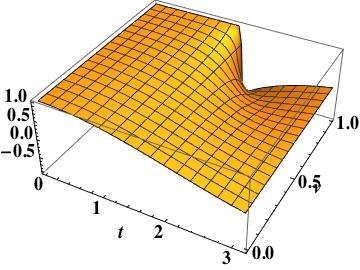
. The phase error can be similarly treated, \alpha \approx 1 + \frac{1}{6}\left(1-2\nu + \nu^2\right) + O\left(\theta^4\right). Please note that the phase error is actually one order higher than I’ve written because of its definition where I have divided

phase-1-contthrough by \nu\theta. The last bit of analysis we conduct is to make an estimate of the rate of convergence as a function of the mesh spacing and CFL number. Given the symbol we can compute the error E=A - \exp\left(-\imath \nu\theta\right). We then compute the error with a refined grid by a factor of two and note that it must applied twice to get the solution to the same point in time. The error for the refined calculation is E_{\frac{1}{2}} = A_{\frac{1}{2}} - \exp \left( - \frac{\imath \nu \theta}{2} \right), which is squared to account for two time steps being taken to get to the same simulation time, E_{\frac{1}{2}}:=E_{\frac{1}{2}}^2 .Given these errors the local rate of convergence is simple, n = \log\left(\left|E\right|/\left|E_\frac{1}{2}\right| \right)/log\left(2\right)
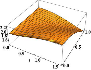
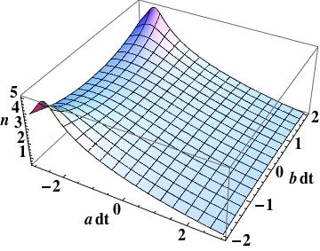
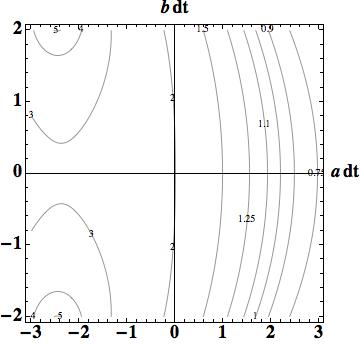
. We can then plot the function where we see that the convergence rate deviates significantly from one (the expected value) for finite values of \theta and \nu.

conv-rate-1We can now apply the same machinery to more complex schemes. Our first example is the time-space coupled version of Fromm’s scheme, which is a second-order method. Conducting the analysis is largely a function of writing the numerical scheme in Mathematica much in the same fashion we would use to write the method into a computer code.

The first version of Fromm’s scheme uses a combined space time differencing introduced by Lax-Wendroff implemented using a methodology similar to Richtmyer’s two-step scheme, which makes the steps clear. First, define a cell-centered slope s_j^n =\frac{1}{2}\left( u_{j+1}^n - u_{j-1}^n\right) and then use this to define a edge-centered, time-centered value, u_{j+1/2}^{n+1/2} = u_j^n + \frac{1}{2}\left(1 - \nu\right) s_j^n. This choice has a “build-in” upwind bias. If the velocity in the equation were oriented oppositely, this choice would be u_{j+1/2}^{n+1/2} = u_{j+1}^n - \frac{1}{2}\left(1 - \nu\right)s_{j+1}^n instead (\nu<0). Now we can write the update for the cell-centered variables as u_j^{n+1} = u_j^n - \nu\left(u_{j+1/2}^{n+1/2} - u_{j-1/2}^{n+1/2}\right), substitute in the Fourier transform and apply all the same rules as for the first-order upwind method.

Just note that in the Mathematica the slope, and edge variables are defined as general functions of the mesh index j and the substitution is accomplished without any pain. This property is essential for analyzing complicated methods that effectively have very large or complex stencils.

amp-2-contphase-2conv-rate-2

The results then follow as before. We can plot the amplitude and phase error easily and the first thing we should notice is the radical improvement over the first-order method, particularly the amplification error at large wavenumbers (i.e., the grid scale). We can go further and use the Taylor series expansion to express the formal accuracy for the amplification and phase error. The amplification error is two orders higher than upwind and is \left| A \right| \approx 1
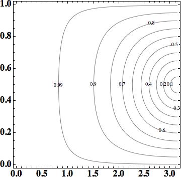
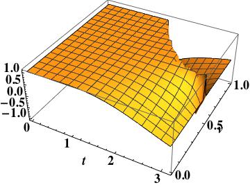
. The phase error is smaller than the upwind scheme, but the same order, \alpha\approx 1. This is the leading order error in Fromm’s scheme.

We can finish by plotting the convergence rate as a function of finite time step and wavenumber. Unlike the upwind scheme as the wavenumber approaches one the rate of convergence is larger than the formal order of accuracy.

The Mathematica commands used to conduct the analysis above:

(* 1st order 1-D *)

U[j_] := T[j]

U1[j_] := U[j] – v (U[j] – U[j – 1])

sym = 1/2 U[0] + 1/2 U1[0] – v/2 (U1[0] – U1[-1]);

T[j_] := Exp[I j t]

Series[sym – Exp[-I v t], {t, 0, 5}]

Simplify[sym]

Sym[v_, t_] := 1/2 E^(-2 I t) (-2 E^(I t) (-1 + v) v + v^2 + E^(2 I t) (2 – 2 v + v^2))

rg1 = Simplify[ComplexExpand[Re[sym]]];

ig1 = Simplify[ComplexExpand[Im[sym]]];

amp1 = Simplify[Sqrt[rg1^2 + ig1^2]];

phase1 = Simplify[ ArcTan[-ig1/rg1]/(v t)];

Series[amp1, {t, 0, 5}]

Series[phase1, {t, 0, 5}]

Plot3D[amp1, {t, 0, Pi}, {v, 0, 1}, AxesLabel -> {t, v}, LabelStyle -> Directive[18, Bold, Black]]

Export[“amp-1.jpg”, %]

ContourPlot[amp1, {t, 0, Pi}, {v, 0, 1}, PlotPoints -> 250, Contours -> {0.1, 0.2, 0.3, 0.4, 0.5, 0.6, 0.7, 0.8, 0.9, 0.99, 1}, ContourShading -> False, Axes -> {True, True}, AxesLabel -> {t, v}, ContourLabels -> All, LabelStyle -> Directive[18, Bold, Black]]

Export[“amp-1-cont.jpg”, %]

Plot3D[phase1, {t, 0, Pi}, {v, 0, 1}, AxesLabel -> {t, v}, LabelStyle -> Directive[18, Bold, Black]]

Export[“phase-1.jpg”, %]

ContourPlot[phase1, {t, 0, Pi}, {v, 0, 1}, PlotPoints -> 250, Contours -> {-1, -0.5, -0.25, 0, 0.25, 0.5, 0.75, 0.9, 0.99, 1, 1.25, 1.5}, ContourShading -> False, Axes -> {True, True}, AxesLabel -> {t, v}, ContourLabels -> All, LabelStyle -> Directive[18, Bold, Black]]

Export[“phase-1-cont.jpg”, %]

err = Sym[v, t] – Exp[-I v t];

err2 = Sym[v, t/2]^2 – Exp[-I v t];

Plot3D[Log[Abs[err]/Abs[err2]]/Log[2], {t, 0.01, Pi/2}, {v, 0, 1}, AxesLabel -> {t, v}, LabelStyle -> Directive[18, Bold, Black]]

Export[“conv-rate-1.jpg”, %]

ContourPlot[Log[Abs[err]/Abs[err2]]/Log[2], {t, 0, Pi}, {v, 0, 1}, PlotPoints -> 250, Contours -> {0.5, 0.75, 0.9, 0.95, 0.99}, ContourShading -> False, Axes -> {True, True}, AxesLabel -> {t, v}, ContourLabels -> All, LabelStyle -> Directive[18, Bold, Black]]

Plot3D[Abs[sym/Exp[-I v t]], {t, 0, Pi}, {v, 0, 5}]

ContourPlot[ If[Abs[sym/Exp[-I v t]] <= 1, Abs[sym/Exp[-I v t]], 0], {t, 0, Pi}, {v, 0, 5}, PlotPoints -> 250, Contours -> {0.1, 0.25, 0.5, 0.75, 0.9, 1}, ContourShading -> False, Axes -> {True, True}, AxesLabel -> {t, v}, ContourLabels -> All, LabelStyle -> Directive[18, Bold, Black]]

errs = Sym[v, t/2]^2 – Sym[v, t];

errs2 = Sym[v, t/4]^4 – Sym[v, t/2]^2;

Plot3D[Log[Abs[errs]/Abs[errs2]]/Log[2], {t, 0.01, Pi/2}, {v, 0, 1}]

errt = Sym[v/2, t]^2 – Sym[v, t];

errt2 = Sym[v/4, t]^4 – Sym[v/2, t]^2;

Plot3D[Log[Abs[errt]/Abs[errt2]]/Log[2], {t, 0, Pi/2}, {v, 0, 1}]

(* classic fromm *)

U[j_] := T[j]

S[j_] := 1/2 (U[j + 1] – U[j – 1])

Ue[j_] := U[j] + 1/2 S[j] (1 – v)

sym2 = U[0] – v (Ue[0] – Ue[-1]);

T[j_] := Exp[I j t]

Series[sym2 – Exp[-I v t], {t, 0, 5}];

Simplify[Normal[%]];

Collect[Expand[Normal[%]], t]

Simplify[sym2]

Sym2[v_, t_] := 1/32 E^(-4 I t) (v^2 – 10 E^(I t) v^2 + E^(6 I t) v^2 + 2 E^(5 I t) v (-4 + 3 v) – 4 E^(3 I t) v (-10 + 7 v) + E^(2 I t) v (-8 + 31 v) – E^(4 I t) (-32 + 24 v + v^2))

rg2 = Simplify[ComplexExpand[Re[sym2]]];

ig2 = Simplify[ComplexExpand[Im[sym2]]];

amp2 = Simplify[Sqrt[rg2^2 + ig2^2]];

phase2 = Simplify[ ArcTan[-ig2/rg2]/(v t)];

Series[amp2, {t, 0, 5}]

Series[phase2, {t, 0, 5}]

Plot3D[amp2, {t, 0, Pi}, {v, 0, 1}, AxesLabel -> {t, v}, LabelStyle -> Directive[18, Bold, Black]]

Export[“amp-2.jpg”, %]

ContourPlot[amp2, {t, 0, Pi}, {v, 0, 1}, PlotPoints -> 250, Contours -> {0.1, 0.2, 0.3, 0.4, 0.5, 0.6, 0.7, 0.8, 0.9, 0.99, 1}, ContourShading -> False, Axes -> {True, True}, AxesLabel -> {t, v}, ContourLabels -> All, LabelStyle -> Directive[18, Bold, Black]]

Export[“amp-2-cont.jpg”, %]

Plot3D[phase2, {t, 0, Pi}, {v, 0, 1}, AxesLabel -> {t, v}, LabelStyle -> Directive[18, Bold, Black]]

Export[“phase-2.jpg”, %]

ContourPlot[phase2, {t, 0, Pi}, {v, 0, 1}, PlotPoints -> 250, Contours -> {-1, -0.5, -0.25, 0, 0.25, 0.5, 0.75, 0.9, 0.99, 1, 1.25, 1.5}, ContourShading -> False, Axes -> {True, True}, AxesLabel -> {t, v}, ContourLabels -> All, LabelStyle -> Directive[18, Bold, Black]]

Export[“phase-2-cont.jpg”, %]

err = Sym2[v, t] – Exp[-I v t];

err2 = Sym2[v, t/2]^2 – Exp[-I v t];

Plot3D[Log[Abs[err]/Abs[err2]]/Log[2], {t, 0.01, Pi/2}, {v, 0, 1}, AxesLabel -> {t, v}, LabelStyle -> Directive[18, Bold, Black]]

Export[“conv-rate-2.jpg”, %]

ContourPlot[ Log[Abs[err]/Abs[err2]]/Log[2], {t, 0.01, Pi}, {v, 0.01, 1}, PlotPoints -> 250, Contours -> {1, 1.5, 1.75, 1.9, 2, 2.1, 2.2, 2.3, 2.4}, ContourShading -> False, Axes -> {True, True}, AxesLabel -> {t, v}, ContourLabels -> All, LabelStyle -> Directive[18, Bold, Black]]

Export[“conv-rate-2-cont.jpg”, %]

ContourPlot[ If[Abs[sym2/Exp[-I v t]] <= 1, Abs[sym2/Exp[-I v t]], 0], {t, 0, Pi}, {v, 0, 1}, PlotPoints -> 250, Contours -> {0.1, 0.25, 0.5, 0.75, 0.9, 1}, ContourShading -> False, Axes -> {True, True}, AxesLabel -> {t, v}, ContourLabels -> All, LabelStyle -> Directive[18, Bold, Black]]

errs = Sym2[v, t] – Sym2[v, t/2]^2;

errs2 = Sym2[v, t/4]^4 – Sym2[v, t/2]^2;

Plot3D[Log[Abs[errs]/Abs[errs2]]/Log[2], {t, 0.01, Pi/2}, {v, 0, 1}, AxesLabel -> {t, v}, LabelStyle -> Directive[18, Bold, Black]]

errt = Sym2[v, t] – Sym2[v/2, t]^2;

errt2 = Sym2[v/4, t]^4 – Sym2[v/2, t]^2;

Plot3D[Log[Abs[errt]/Abs[errt2]]/Log[2], {t, 0.0, Pi/2}, {v, 0, 0.1}]

(* 2nd order Fromm – RK *)

U[j_] := T[j]

S[j_] := 1/2 (U[j + 1] – U[j – 1])

Ue[j_] := U[j] + 1/2 S[j]

U1[j_] := U[j] – v (Ue[j] – Ue[j – 1])

S1[j_] := 1/2 (U1[j + 1] – U1[j – 1])

Ue1[j_] := U1[j] + 1/2 S1[j]

sym2 = 1/2 U[0] + 1/2 U1[0] – v/2 (Ue1[0] – Ue1[-1]);

T[j_] := Exp[I j t]

Series[sym2 – Exp[-I v t], {t, 0, 5}];

Simplify[Normal[%]];

Collect[Expand[Normal[%]], t]

Simplify[sym2]

Sym2[v_, t_] := 1/32 E^(-4 I t) (v^2 – 10 E^(I t) v^2 + E^(6 I t) v^2 + 2 E^(5 I t) v (-4 + 3 v) – 4 E^(3 I t) v (-10 + 7 v) + E^(2 I t) v (-8 + 31 v) – E^(4 I t) (-32 + 24 v + v^2))

rg2 = Simplify[ComplexExpand[Re[sym2]]];

ig2 = Simplify[ComplexExpand[Im[sym2]]];

amp2 = Simplify[Sqrt[rg2^2 + ig2^2]];

phase2 = Simplify[ ArcTan[-ig2/rg2]/(v t)];

Series[amp2, {t, 0, 5}]

Series[phase2, {t, 0, 5}]

Plot3D[amp2, {t, 0, Pi}, {v, 0, 1}, AxesLabel -> {t, v}, LabelStyle -> Directive[18, Bold, Black]]

Export[“amp-2rk.jpg”, %]

ContourPlot[amp2, {t, 0, Pi}, {v, 0, 1}, PlotPoints -> 250, Contours -> {0.1, 0.2, 0.3, 0.4, 0.5, 0.6, 0.7, 0.8, 0.9, 0.99, 1}, ContourShading -> False, Axes -> {True, True}, AxesLabel -> {t, v}, ContourLabels -> All, LabelStyle -> Directive[18, Bold, Black]]

Export[“amp-2rk-cont.jpg”, %]

Plot3D[phase2, {t, 0, Pi}, {v, 0, 1}, AxesLabel -> {t, v}, LabelStyle -> Directive[18, Bold, Black]]

Export[“phase-2rk.jpg”, %]

ContourPlot[phase2, {t, 0, Pi}, {v, 0, 1}, PlotPoints -> 250, Contours -> {-1, -0.5, -0.25, 0, 0.25, 0.5, 0.75, 0.9, 0.99, 1, 1.25, 1.5}, ContourShading -> False, Axes -> {True, True}, AxesLabel -> {t, v}, ContourLabels -> All, LabelStyle -> Directive[18, Bold, Black]]

Export[“phase-2rk-cont.jpg”, %]

err = Sym2[v, t] – Exp[-I v t];

err2 = Sym2[v, t/2]^2 – Exp[-I v t];

Plot3D[Log[Abs[err]/Abs[err2]]/Log[2], {t, 0.01, Pi/2}, {v, 0, 1}, AxesLabel -> {t, v}, LabelStyle -> Directive[18, Bold, Black]]

Export[“conv-rate-2rk.jpg”, %]

ContourPlot[ Log[Abs[err]/Abs[err2]]/Log[2], {t, 0.01, Pi}, {v, 0.01, 1}, PlotPoints -> 250, Contours -> {1, 1.5, 1.75, 1.9, 2, 2.1, 2.2, 2.3, 2.4}, ContourShading -> False, Axes -> {True, True}, AxesLabel -> {t, v}, ContourLabels -> All, LabelStyle -> Directive[18, Bold, Black]]

Export[“conv-rate-2rk-cont.jpg”, %]

ContourPlot[ If[Abs[sym2/Exp[-I v t]] <= 1, Abs[sym2/Exp[-I v t]], 0], {t, 0, Pi}, {v, 0, 1.5}, PlotPoints -> 250, Contours -> {0.1, 0.25, 0.5, 0.75, 0.9, 1}, ContourShading -> False, Axes -> {True, True}, AxesLabel -> {t, v}, ContourLabels -> All, LabelStyle -> Directive[18, Bold, Black]]

errs = Sym2[v, t] – Sym2[v, t/2]^2;

errs2 = Sym2[v, t/4]^4 – Sym2[v, t/2]^2;

Plot3D[Log[Abs[errs]/Abs[errs2]]/Log[2], {t, 0.01, Pi/2}, {v, 0, 1}]

errt = Sym2[v, t] – Sym2[v/2, t]^2;

errt2 = Sym2[v/4, t]^4 – Sym2[v/2, t]^2;

Plot3D[Log[Abs[errt]/Abs[errt2]]/Log[2], {t, 0.0, Pi/2}, {v, 0, 0.1}]

Conducting von Neumann stability analysis

15 Tuesday Jul 2014

Posted by Bill Rider in Uncategorized

≈ 4 Comments

In order to avoid going on another (epic) rant this week, I’ll change gears and touch upon a classic technique for analyzing the stability of numerical methods along with extensions or the traditional approach.

Before diving into partial differential equations, I thought it would be beneficial to analyze the stability of ordinary differential equation integrators first. This provides the basis of the approach. Next I will show how the analysis proceeds for an important second-order method for linear advection. I will close with providing the analysis of second-order discontinuous Galerkin methods, which introduce an important wrinkle on the schemes. I will close by producing the Mathematica commands used to give the results.

It is always good to have references that can be read for detail and explanation than I will give a few seminal ones here:

* Ascher, Uri M., and Linda R. Petzold. Computer methods for ordinary differential equations and differential-algebraic equations. Vol. 61. Siam, 1998.

* Durran, Dale R. Numerical methods for wave equations in geophysical fluid dynamics. No. 32. Springer, 1999.

* LeVeque, Randall J., and Randall J. Le Veque. Numerical methods for conservation laws. Vol. 132. Basel: Birkhäuser, 1992.

* LeVeque, Randall J. Finite volume methods for hyperbolic problems. Vol. 31. Cambridge university press, 2002.

* Strikwerda, John C. Finite difference schemes and partial differential equations. Siam, 2004.

Let’s jump into the analysis of ODE solvers by looking at a fairly simple method, the forward Euler method. We can write the solver for a simple ODE, u_t =\lambda u, as simply u^{n+1} = u^n + \Delta t \lambda u^n. We take the right hand side \lambda = a + b \imath, and do some algebra. We have several principal goals, establish conditions for stability, accuracy, and overall behavior of the method.

For stability we determine how much the value of the solution is amplified by the action of the integration scheme, u^{n+1}= A u^n = u^n + \Delta t \lambda u^n, we remove the variable and call the result the “symbol’’ of the integrator, A = 1 + \Delta t \lambda , we then solve for A=\left| A \right| \exp(-\imath \alpha) then take its magnitude, = \left| A \right|, being less than one for stability. We can write down this answer explicitly =\left| A \right|\ = \sqrt{(1+\Delta t a)^2 + (\Delta t b)^2}
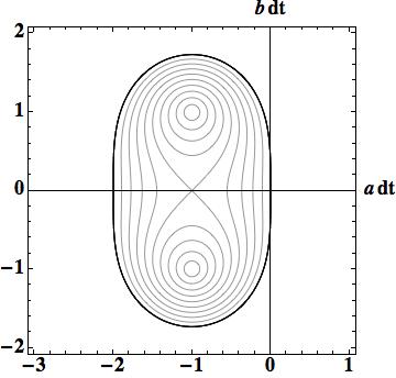
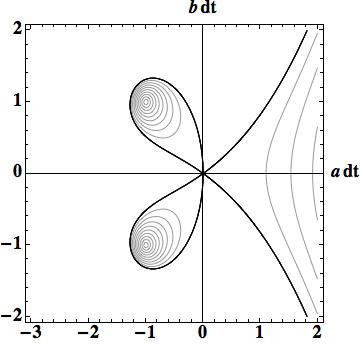
. We can also plot this result easily (see the commands I used in Mathematica at the end of the post).  On all the plots the horizontal axis is the real values a \Delta t and the vertical axis is the imaginary values b\Delta t.


This plot just includes the values where they amplitude of the symbol is less than or equal to one.forwardEuler

Next we look at accuracy using a Taylor series expansion. The Taylor series is simple given the analytical solution to the ODE, u(t)=\exp(\lambda t), and the Taylor series expansion is classical, \exp(\lambda t)\approx 1 + t \lambda + \frac{1}{2}(\lambda t)^2 + \frac{1}{6}(\lambda t)^3 + O(t^4). We simply subtract this Taylor series from the symbol of the operator and look at the remainder, $\latex E= \frac{1}{2}(\lambda \Delta t)^2+ O(\Delta t^3)$, where the time has been replaced by the time step size.

The last couple of twists can add some significant texture to the behavior of the integration scheme. We can plot the “order stars’’ which shows whether the numerical scheme changes the amplitude of the answer more or less than the exact operator. These are call stars because they start to show star-like shapes for higher order methods (mostly starting at third- and higher order accuracy). He is the plot for forward Euler.

forwardEuler-star

The last thing we will examine for the forward Euler scheme is the order of accuracy you should see during a time step refinement study as part of a verification exercise. Usually this is thought of as being the same as the order of the numerical scheme, but for a finite time step size the result deviates from the analytical order substantially. Computing this is really quite simple, one simply compute the symbol of the operator for half the time step size \Delta t/2, A_\frac{1}{2} for two time steps (so that the time ends up at the same place as you get for a single step with \Delta t. This is simply the square of the operator at the smaller time step size. To get the order of accuracy you take the operators and subtract the exact solution, take the absolute value of the result, then compute the order of accuracy like usual verification,

a=\frac{\log\frac{\left|A-\exp(\lambda \Delta t)\right|}{\left| A_\frac{1}{2}^2 -\exp(\lambda \Delta t )\right|} }{\log(2)}.

We can plot the result easily with Mathematica. It is notable how different from the asymptotic value of one the results are for reasonable, but finite values of \Delta t. As the operator becomes unstable, the convergence rate actually becomes very large. This is a word of warning to the practitioner that very high rates of convergence can actually be a very bad sign for a calculation.

forwardEuler-order

forwardEuler-order-contourLook for

We can now examine a second-order method with relative ease.  Doing the analysis is akin to writing a computer code albeit symbolically.  The second-order is using a predictor-corrector format where a half step is taken using forward Euler and this result is used to advance the solution the full step. This is an improved forward Euler method.  It is explicit in that the solution can be evaluated solely in terms of the initial data. The scheme is the following: u^{n+1/2} = u^n + \Delta t/2 \lambda u^n for the predictor, and u^{n+1} = u^n + \Delta t \lambda u^{n+1/2}.  The symbol is computed as before giving A=1+ \Delta t \lambda \left( 1+\Delta t \lambda /2\right).  Getting the full properties of the method now just requires “turning the crank’’ as we did for the forward Euler scheme.

The truncation error has gained an order of accuracy and now is E= \frac{1}{6}(\lambda \Delta t)^3+ O(\Delta t^4).

The stability plot is more complex giving a larger region for the stability particularly along the imaginary axis.rk2

The order star looks much more like a star.

rk2-star

Finally the convergence rate plot is much less pathalogical although some of the same conclusions can be drawn from the behavior where the scheme is unstable (giving the very large convergance rates).

rk2-orderrk2-order-contour

We will finish this week’s post by turning our attention to a second order implicit scheme, the backwards differentiation formula (BDF).  Everything will follow from the previous two example, but the scheme adds an important twist (or two).  The first twist is that the method is implicit, meaning that the left and right hand sides of the method are coupled, and the second is that the method depends on three time levels of data, not two as the first couple of methods.

The update for the method is written \frac{3}{2} u^{n+1}-2 u^n +\frac{1}{2} u^{n-1} = \Delta t \lambda u^{n+1}, and the amplification is now a quadratic equation, \left( \frac{3}{2} - \Delta t \lambda\right) A^2 -2 A +\frac{1}{2} = 0  with two roots. One of these roots will have a Taylor series expansion that demonstrates second-order accuracy for the scheme, the other will not. The inaccurate root must still be stable for the scheme to be stable. The accurate root is

A=\frac{-2-\sqrt{1+\Delta t \lambda}}{\Delta t \lambda -3}

with a error of E= \frac{1}{3}(\lambda \Delta t)^3+ O(\Delta t^4).

The second inaccurate root is also called spurious and has the form

bdf2A=\frac{-2+\sqrt{1+\Delta t \lambda}}{\Delta t \lambda -3}.

The stability of the scheme requires taking the maximum of the magnitude of both roots.

Using the accurate root we can examine the order star, and the rate of convergence of the method as before.


Next week we will look at a simple partial differential equation analysis, which adds new wrinkles.

While this sort of analysis can be done by hand, the greatest utility can be achbdf2-order-contourbdf2-starbdf2-orderieved by using symbolic or numerical packages such as Mathematica. Below I’ve included the Mathematica code used for the analyses given above.

Soln = Collect[Expand[Normal[Series[Exp[h L], {h, 0, 6}]]], h]

(* Forward Euler *)

a =.; b =.

A = 1 + h L

Aab2 = (1 + h L/2 )^2

Collect[Expand[Normal[Series[A, {h, 0, 6}]]], h];

Soln – %

L = ( a + b I)/h;

ContourPlot[If[Abs[A] < 1, -Abs[A], 1], {a, -3, 1}, {b, -2, 2},
PlotPoints -> 250,
Contours -> {-0.1, -0.2, -0.3, -0.4, -0.5, -0.6, -0.7, -0.8, -0.9},
ContourShading -> False, Axes -> {True, True},
AxesLabel -> {a dt, b dt}, LabelStyle -> Directive[18, Bold, Black]]

Export[“forwardEuler.jpg”, %]

“forwardEuler.jpg”

ContourPlot[
If[Abs[A]/Abs[Exp[a + b I]] < 1, -Abs[A]/Abs[Exp[a + b I]],
1], {a, -3, 2}, {b, -2, 2}, PlotPoints -> 250,
Contours -> {-0.1, -0.2, -0.3, -0.4, -0.5, -0.6, -0.7, -0.8, -0.9},
ContourShading -> False, Axes -> {True, True},
AxesLabel -> {a dt, b dt}, LabelStyle -> Directive[18, Bold, Black]]

Export[“forwardEuler-star.jpg”, %]

“forwardEuler-star.jpg”

Plot3D[Log[Abs[A – Exp[a + b I]]/Abs[Aab2 – Exp[a + b I]]]/
Log[2], {a, -3, 3}, {b, -2, 2}, PlotPoints -> 100,
AxesLabel -> {a dt, b dt, n},
LabelStyle -> Directive[18, Bold, Black], PlotRange -> All]

Export[“forwardEuler-order.jpg”, %]

“forwardEuler-order.jpg”

ContourPlot[
Log[Abs[A – Exp[a + b I]]/Abs[Aab2 – Exp[a + b I]]]/Log[2], {a, -3,
3}, {b, -2, 2}, PlotPoints -> 250,
Contours -> {0, 0.25, 0.5, 0.75, 0.9, 1, 1.1, 1.25, 1.5, 2, 3, 4, 5,
10}, ContourShading -> False, ContourLabels -> All,
Axes -> {True, True}, AxesLabel -> {a dt, b dt},
LabelStyle -> Directive[18, Bold, Black], PlotRange -> All]

Export[“forwardEuler-order-contour.jpg”, %]

“forwardEuler-order-contour.jpg”

ContourPlot[
If[Abs[A] < 1, Abs[A – Exp[a + b I]]/Abs[Aab2 – Exp[a + b I]],
0], {a, -3, 2}, {b, -2, 2}, PlotPoints -> 250,
Contours -> {2, 2.5, 3, 3.5, 4}, ContourShading -> False,
Axes -> {False, True}]

Plot3D[Abs[A – Exp[a + b I]]/Abs[Aab2 – Exp[a + b I]], {a, -3,
3}, {b, -2, 2}, PlotPoints -> 100]

ContourPlot[
If[Abs[A]/Abs[Exp[a + b I]] < 1, -Abs[A]/Abs[Exp[a + b I]],
1], {a, -3, 2}, {b, -2, 2}, PlotPoints -> 250,
Contours -> {-0.1, -0.2, -0.3, -0.4, -0.5, -0.6, -0.7, -0.8, -0.9},
ContourShading -> False, Axes -> {False, True}]

(* RK 2 *)

L =.

A1 = 1 + 1/2 h L

A = 1 + h L A1

A12 = 1 + 1/4 h L;

Aab2 = (1 + h L A12/2 )^2

Collect[Expand[Normal[Series[A, {h, 0, 6}]]], h] – Soln

L = ( a + b I)/h;

ContourPlot[If[Abs[A] < 1, -Abs[A], 1], {a, -3, 1}, {b, -2, 2},
PlotPoints -> 250,
Contours -> {-0.1, -0.2, -0.3, -0.4, -0.5, -0.6, -0.7, -0.8, -0.9},
ContourShading -> False, Axes -> {True, True},
AxesLabel -> {a dt, b dt}, LabelStyle -> Directive[18, Bold, Black]]

Export[“rk2.jpg”, %]

ContourPlot[
If[Abs[A]/Abs[Exp[a + b I]] < 1, -Abs[A]/Abs[Exp[a + b I]],
1], {a, -3, 2}, {b, -2, 2}, PlotPoints -> 250,
Contours -> {-0.1, -0.2, -0.3, -0.4, -0.5, -0.6, -0.7, -0.8, -0.9},
ContourShading -> False, Axes -> {True, True},
AxesLabel -> {a dt, b dt}, LabelStyle -> Directive[18, Bold, Black]]

Export[“rk2-star.jpg”, %]

Plot3D[Log[Abs[A – Exp[a + b I]]/Abs[Aab2 – Exp[a + b I]]]/
Log[2], {a, -3, 3}, {b, -2, 2}, PlotPoints -> 100,
AxesLabel -> {a dt, b dt, n},
LabelStyle -> Directive[18, Bold, Black], PlotRange -> All]

Export[“rk2-order.jpg”, %]

ContourPlot[
Log[Abs[A – Exp[a + b I]]/Abs[Aab2 – Exp[a + b I]]]/Log[2], {a, -3,
3}, {b, -2, 2}, PlotPoints -> 250,
Contours -> {0, 0.25, 0.5, 0.75, 0.9, 1, 1.1, 1.25, 1.5, 2, 3, 4, 5,
10}, ContourShading -> False, ContourLabels -> All,
Axes -> {True, True}, AxesLabel -> {a dt, b dt},
LabelStyle -> Directive[18, Bold, Black], PlotRange -> All]

Export[“rk2-order-contour.jpg”, %]

(* BDF 2 *)

A =.

L =.

Solve[3/2 A^2 – 2 A + 1/2 == h A^2 L, A]

A1 = (-2 – Sqrt[1 + 2 h L])/(-3 + 2 h L); A2 = (-2 + Sqrt[
1 + 2 h L])/(-3 + 2 h L);

Solve[3/2 A^2 – 2 A + 1/2 == 1/2 h A^2 L, A]

Aab2 = ((-2 – Sqrt[1 + h L])/(-3 + h L) )^2;

Collect[Expand[Normal[Series[A1, {h, 0, 6}]]], h] – Soln

Collect[Expand[Normal[Series[A2, {h, 0, 6}]]], h] – Soln

L = ( a + b I)/h;

ContourPlot[
If[Max[Abs[A1], Abs[A2]] < 1, -Max[Abs[A1], Abs[A2]], 1], {a, -8,
6}, {b, -5, 5}, PlotPoints -> 250,
Contours -> {-0.1, -0.2, -0.3, -0.4, -0.5, -0.6, -0.7, -0.8, -0.9},
ContourShading -> False, Axes -> {True, True},
AxesLabel -> {a dt, b dt}, LabelStyle -> Directive[18, Bold, Black]]

Export[“bdf2.jpg”, %]

ContourPlot[

If[Abs[A1]/Abs[Exp[a + b I]] < 1, -Abs[A1]/Abs[Exp[a + b I]],
1], {a, -3, 2}, {b, -2, 2}, PlotPoints -> 250,
Contours -> {-0.1, -0.2, -0.3, -0.4, -0.5, -0.6, -0.7, -0.8, -0.9},
ContourShading -> False, Axes -> {True, True},
AxesLabel -> {a dt, b dt}, LabelStyle -> Directive[18, Bold, Black]]

Export[“bdf2-star.jpg”, %]

Plot3D[Log[Abs[A1 – Exp[a + b I]]/Abs[Aab2 – Exp[a + b I]]]/
Log[2], {a, -8, 6}, {b, -5, 5}, PlotPoints -> 100,
AxesLabel -> {a dt, b dt, n},
LabelStyle -> Directive[18, Bold, Black]]

Export[“bdf2-order.jpg”, %]

ContourPlot[
Log[Abs[A1 – Exp[a + b I]]/Abs[Aab2 – Exp[a + b I]]]/Log[2], {a, -8,
6}, {b, -5, 5}, PlotPoints -> 250,
Contours -> {-1, 0, 0.5, 0.9, 1, 1.1, 1.5, 2, 5, 10},
ContourShading -> False, ContourLabels -> All, Axes -> {True, True},
AxesLabel -> {a dt, b dt}, LabelStyle -> Directive[18, Bold, Black],
PlotRange -> All]

Export[“bdf2-order-contour.jpg”, %]


The 2014 SIAM Annual Meeting, or what is the purpose of Applied Mathematics?

11 Friday Jul 2014

Posted by Bill Rider in Uncategorized

≈ 1 Comment

Donald Knuth -“If you find that you’re spending almost all your time on theory, start turning some attention to practical things; it will improve your theories. If you find that you’re spending almost all your time on practice, start turning some attention to theoretical things; it will improve your practice.”

This week I visited Chicago for the 2014 SIAM Annual Meeting (Society for Industrial and Applied Mathematics). It was held at tPalmer-house-lobby-final-larger-e1380753290284he Palmer House, which is absolutely stunning venue swimming in old-fashioned style and grandeur. It is right around the corner from Millennium Park, which is one of the greatest Urban green spaces in existence, which itself is across the street from the Art Institute. What an inspiring setting to hold a meeting. Chicago itself is one of the great American cities with a vibrant downtown and numerous World-class sites.

The meeting included a lot of powerful content and persuasive applications of applied mathematics. Still some of the necessary gravity for the work seems to be missing from the overall dialog with most of the research missing the cutting edge of reality. There just seems to be a general lack of vitality and impCloud_Gate_at_Millenium_Park_Chicago_aug_2007_2__soul-amportance to the overall scientific enterprise, and applied mathematics is suffering likewise. This isn’t merely the issue of funding, which is relatively dismal, but overall direction and priority. In total, we aren’t asking nearly enough from science, and mathematics is no different. The fear of failure is keeping us from collectively attacking society’s most important problems. The distressing part of all of this is the importance and power of applied mathematics and the rigor it brings to science as a whole. We desperately need some vision moving forward.

The importance of applied mathematics to the general scientific enterprise should not be in doubt, but it is. I sense a malaise in the entire scientific field stemming from the overall lack of long-term perspective for the Nation as a whole. Is the lack of vitality specific to this field, or a general description of research?

I think it is useful to examine how applied mathematics can be an important force for order, confidence and rigor in science. Indeed applied mathematics can be a powerful force to aid the practice of science. For example there is the compelling example of compressed sensing (told in the Wired article ct-foihttp://www.wired.com/2010/02/ff_algorithm/). The notion that the L1 norm had magical properties to help unveil the underlying sparsity in objects was an old observation, but not until mathematical rigor was put in place to underpin this observation did the practice take off. There is no doubt that the entire field exploded in interest when the work of Candes, Tao and Donoho put a rigorous face on the magical practice of regularizing a problem with the L1 norm. It shouldn’t be under-estimated that the idea came at the right time; this is a time when we are swimming in data from an increasing array of sources, and compressed sensing conceptually provides a powerful tool for dealing with this. At the same time, the lack of rigor limited the interest in the technique prior to 2004 or 2005.

One of the more persuasive cases where applied mathematics has provided a killer theory is 41CvwPJb73L
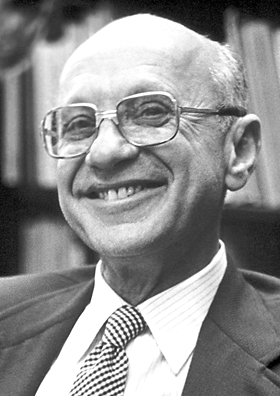
the work of Peter Lax on hyperbolic conservation laws. He laid the groundwork for stunning progress in modeling and simulating with confidence and rigor. There are other examples such as the mathematical order and confidence of the total variation diminishing theory of Harten to power the penetration of high-resolution methods into broad usage for solving hyperbolic PDEs. Another example is the relative power and confidence brought to the solution of ordinary differential equations, or numerical linear algebra by the mathematical rigor underlying the development of software. These are examples where the presence of applied mathematics makes a consequential and significant difference in the delivery of results with confidence and rigor. Each of these is an example of how mathematics can unleash a capability in truly “game-changing” ways. A real concern is why this isn’t happening more broadly or in targeted manner.

I started the week with a tweet of Richard Hamming’s famous quote – “The purpose of computing is insight, not numbers.” During one of the highlight talks of the meeting we received a modification of that maxim by the lecturer Leslie Greengard,

“The purpose of computing is to get the right answer”.

A deeper question with an uncertainty quantification spin would be “which right answer?” My tweet in response to Greengard then said

“The purpose of computing is to solve more problems than you create.”

This entire dialog is the real topic of the post. Another important take was by Joseph Teran on scientific computing in special effects for movies. Part of what sat wrong with me was the notion that looking right becomes equivalent to being right. On the other hand the perception and vision of something like turbulent fluid flow shouldn’t be underestimated. If it looks right there is probably something systematic lying beneath the superficial layer of entertainment. The fact that the standard for turbulence modeling for science and movies might be so very different should be startling. Ideally the two shouldn’t be that far apart. Do special effects have something to teach us? Or something worthy of explanation? I think these questions make mathematicians very uncomfortable.

climate-modelIf it makes you uncomfortable, it might be a good or important thing to ask. That uncomfortable question might have a deep answer that is worth attacking. I might prefer to project this entire dialog into the broader space of business practice and advice. This might seem counter-intuitive, but the broader societal milieu today is driven by business.

“Don’t find customers for your products, find products for your customers.” ― Seth Godin

One of the biggest problems in the area where I work is the maturity of the field. People simply don’t think about what the entire enterprise is for. Computational simulation and modeling is about using a powerful tool to solve problems. The computer allows certain problem solving approaches to be used that aren’t possible with out it, but the problem solving is the central aspect. I believe that the fundamental utility of modeling and simulation is being systematically taken for granted. The centrality of the problem being solved has been lost and replaced by simpler, but far less noble pursuits. The pursuit of computational power has become a fanatical desire that has swallowed the original intent. Those engaging in this pursuit have generally good intentions, but lack the well-rounded perspective on how to achieve success. For example, the computer is only one small piece of the toolbox and to use a mathematical term, necessary, but gloriously insufficient.

jaguar-7Currently the public policy is predicated upon the notion that a bigger faster computer provides an unambiguously better solution. Closely related to this notion is a technical term in computational modeling and mathematics known as convergence. The model converges or approaches a solution as more computational resource is applied. If you do everything right this will happen, but as problems become more complex you have to do a lot of things right. The problem is that we don’t have the required physical or mathematical knowledge to have the expectation of this in many cases. These are the very cases that we use to justify the purchase of new computers.

The guarantee of convergence ought to be at the very heart of where applied mathematics is striving; yet the community as a whole seems to be shying away from the really difficult questions. Today too much applied mathematics focuses upon simple model equations that are well behaved mathematically, but only capture cartoon aspects of the real problems facing society. Over the past several decades focused efforts on attacking these real problems have retreated. This retreat is part of the overall base of fear of failure in research. Despite the importance of these systems, we are not pushing the boundaries of knowledge to envelop them with better understanding. Instead we spend effort redoubling our efforts to understand simple model equations. This lack of focus on real problems is one of the deepest and most troubling aspects of the current applied mathematics community.

We have evolved to the point in computational modeling and simulation where today we don’t actually solve problems any more. We have developed useful abstractions that have taken the place of the actual problem solving. In a deep sense we now solve cartoonish versions of actual problems. These cartoons allow the different sub-fields to work independently of one another. For example, the latest and greatest computers require super high-resolution 3-D (or 7-D) solutions to the model problems. Actual problem solving rarely (never) works this way. If the problem can be solved in a lower-dimensional manner, it is better. Actual problem solving always starts simple and builds its way up. We start in one dimension and gain experience, run lots of problems, add lots of physics to determine what needs to be included in the model. The mantra of the modern day is to short-circuit this entire approach and jump to add in all the physics, and all the dimensionality, and all the resolution. It is the recipe for disaster, and that disaster is looming before us.

The reason for this is a distinct lack of balance in how we are pursing the objective of better modeling and simulation. To truly achieve progress we need a return to a balanced problem solving perspective. While this requires attention to computing, it also requires physical theory and experiment, deep engineering, computer science, software engineering, mathematics, and physiology. Right now, aside from computers themselves and computer science, the endeavor is woefully out of balance. We have made experiments almost impossible to conduct, and starved the theoretical aspects of science in both physics and mathematics.

Take our computer codes as an objective example of what is occurring. The modeling and simulation is no better than the physical theory and the mathematical approximations used. In many cases these ideas are now two or three decades old. In a number of cases the theory gives absolutely no expectation of convergence as the computational resource is increased. The entire enterprise is predicated on this assumption, yet it has no foundation in theory! The divorce between what the codes do and what the applied mathematicians at SIAM do is growing. The best mathematics is more and more irrelevant to the codes being run on the fastest computers. Where excellent new mathematical approximations exist they cannot be applied to the old codes because of the fundamental incompatibility of the theories. Despite these issues little or no effort exists to rectify this terrible situation.

Why?

friedman_postcardPart of the reason is our fixation on short-term goals, and inability to invest in long-term ends. This is true in science, mathematics, business, roads, bridges, schools, universities, …

Long-term thinking has gone the way of the dinosaur. It died in the 1970’s. I came across a discussion of one of the key ideas of our time, the perspective that business management is all about maximizing shareholder value. It was introduced in 1976 by Nobel Prize-winning economist, Milton Friedman and took hold like a leech. It arguable that it is the most moronic idea ever in business (“the dumbest idea ever”). Nonetheless it has become the lifeblood of business thought, and by virtue of being a business mantra, lifeblood of government thinking. It has been poisoning the proverbial well ever since. It has become the reason for the vampiric obsession with short-term profits, and a variety of self-destructive business practices. The only “positive” side has been its role in driving the accumulation of wealth within chief executives, and financial services. Stock is no longer held for any significant length of time, and business careers hinge upon the quarterly balance sheet. Whole industries have been ground under the wheels of the quarterly report. Government research in a lemming like fashion has followed suit and driven research to be slaved to the quarterly report too.

Philippine-stock-market-boardThe consequences for the American economy have been frightening. Aside from the accumulation of wealth by upper management, we have had various industries completely savaged by the practice, rank and file workers devalued and fired, and no investment in future value. The stock trading frenzy created by this short-term thinking has driven the creation of financial services that produce nothing of value for the economy, and have succeeded in destabilizing the system. As we have seen in 2008 the results can be nearly catastrophic. In addition, the entire business-government system has become unremittingly corrupt and driven by greed and influence peddling. Corporate R&D used to be a vibrant source of science funding and form a pipeline for future value. Now it is nearly barren with the great corporate research labs fading memories. The research that is funded is extremely short-term focused and rarely daring or speculative. The sorts of breakthroughs that have become the backbone of the modern economy no longer get any attention.

The government has been similarly infested as anything that is “good” business practice is “good” for government management. Science is no exception. We now have to apply similar logic to our research and submit quarterly reports. Similar to business we have had to strip mine the future and inflate our quarterly bottom line. The result has been a systematic devaluing of the future. The national leadership has adopted the short-term perspective whole cloth.

At least in some quarters there is recognition of this trend and a push to reverse this trend. It is going to be a hard path to reversing the problem as the short-term focus has been the “goose that laid the golden egg” for many. These ideas have also distorted the scientific enterprise in many ways. The government’s and business’ investment in R&D has become inherently shortsighted. This has caused the whole approach to science to become radically imbalanced. Computational modeling and simulation is but one example that I’m intimately familiar with. It is time to turn things around.

Irrational fear is killing our future?

04 Friday Jul 2014

Posted by Bill Rider in Uncategorized

≈ Leave a comment

“Fear is the mind-killer.” — Frank Herbert

The United States likes to think of itself as a courageous country (a country full of heros). This picture is increasingly distant from the reality of a society of cowards who are almost scared of their own shadows. Why? What is going on in our society to drive trend to be scared of everything?Calling the United States a bunch of cowards seems BaldEaglerather hyperbolic, and it is. The issue is that the leadership of the nation is constantly stoking the fires of irrational fear as a tool to drive political goals. By failing to aspire toward a spirit of shared sacrifice and duty, we are creating a society that looks to avoid anything remotely dangerous or risky. The consequences of this cynical form of gamesmanship are slowly ravaging the United States’ ability to be a dynamic force for anything good. In the process we are sapping the vitality that once brought the nation to the head of the international order. In some ways this trend is symptomatic of our largess as the sole military and economic superpower of the last half of the 20th Century. The fear is drawn from the societal memory of our fading roll in the World, and the evolution away from the mono-polar power we once represented.

Where is the national leadership that calls on citizens to reach for the stars? Where are the voices asking for courage and sacrifice? Once upon a time we had leaders who asked much of us.

“For of those to whom much is given, much is required. “
and
“And so, my fellow Americans: ask not what your country can do for you — ask what you can do for your country.” – John F. Kennedy.

The consequences of this fear go well beyond mere name-calling or implications associated with the psychological aspects of fear, but undermine the ability of the Country to achieve anything of substance, or spend precious resources rationally. The use of fear to motivate people’s choices by politicians is rampant as is the use of fear in managing work. Fear moves people to make irrational choices, and our Nation’s leader whether in government or business want people to choose irrationally in favor of outcomes that benefit those in power. Fear is a powerful way to achieve this. All of this is a serious negative drain on the nation. In almost any endeavor trying to do things you are afraid of leads to diminished performance. One works harder to avoid the negative outcome than achieve the positive one. Fear is an enormous tax on all our efforts, and usually leads to the outcomes that we feared in the first place. We live in a world where broad swaths of public policy are fear-driven. It is a plague on our culture.

Like many of you, my attention has been drawn to the event in Iraq (and Syria) with the onslaught of ISIS. A chorus of fear mongering by politicians bent of scaring the public to support military action to stem the tide of anti-Western faFighters of  al-Qaeda linked Islamic State of Iraq and the Levant parade at Syrian town of Tel Abyadctions in the region has coupled this. Supposedly ISIS is worse than Al Qaeda, and we should be afraid. You are so afraid that you will demand action. In fact that hamburger you are stuffing into your face is a much larger danger to your well being than ISIS will ever be. Worse yet, we put up with the fear-mongers whose fear baiting is aided and abetted by the new media because they see ratings. When we add up the costs, this chorus of fear is savaging us and it is hurting our Country deeply.

“Stop letting your fear condemn you to mediocrity.” ― Steve Maraboli,

We have collectively lost the ability to judge the difference between a real threat and an unfortunate occurrence. Even if we include the loss of life on 9-11 the threat to you due to terrorism is minimal. Despite this reality we expend fast sums of money, time, effort and human lives trying to stop it. It is an abysmal investment of all of these things. We could do so much more with those resources. To make matters worse, the “War on Terror” has distorted our public policy in numerous ways. Stating with the so-called Patriot act we have sacrifice freedom and privacy at the altar of public safety and national security. We create the Department of Homeland Security (a remarkably Soviet sounding name at that), which is a monument to wasting taxpayer money. Perhaps the most remarkable aspect of the DHS is that entering the BinLadenUnited States is now more arduous than entering the former Soviet Union (Russia). This fact ought to absolutely be appalling to the American psyche. Meanwhile, numerous bigger threats go completely untouched by action or effort to mitigate their impact.

For starters as the news media became more interested in ratings than news, they began to amplify the influence of the exotic events. Large, unusual, violent events are ratings gold, and their presence in the news is grossly inflated. The mundane everyday things that are large risks are also boring or depressing, and people would just as soon ignore them. In many cases the mundane everyday risks are huge moneymakers for the owners and advertisers in the media, and they have no interest in killing their cash cow even at the expense of human life (think the medical-industrial complex, and agri-business). Given that people are already horrific at judging statistical risks, these trends have only tended to increase the distance between perceived and actual danger. Politicians know all these things and use them to their advantage. The same things that get ratings for the news grab voter’s attention, and the cynics “leading” the country know it.

TrickyDickWhen did all this start? I tend to think that the tipping point was the mid-1970’s. This era was extremely important for the United States with a number of psychically jarring events taking center stage. The upheaval of the 1960’s had turned society on its head with deep changes in racial and sexual politics. The Vietnam War had undermined the Nation’s innate sense of supremacy while scandal ripped through the government. Faith and trust in the United States took a major hit. At the same time it marked the apex of economic equality with the beginnings of the trends that have undermined it ever since. This underlying lack of faith and trust in institutions has played a key roll in powering our decline. The anti-tax movement that set in motion public policy that drives the growing inequality in income and wealth began then arising from these very forces. These coupled to the insecurities of national defense, gender and race to form the foundation of the modern conservative movement. These fears have been used over and over to drive money and power into the military-intelligence-industrial-complex at a completely irrational rate.

“They who can give up essential liberty to obtain a little temporary safety deserve neither liberty nor safety.” ― Benjamin Franklin

President Bush Renews USA Patriot ActThe so-called Patriot Act is an exemplar of the current thinking. There seems to be no limit to the amount of freedom American will sacrifice to gain a marginal and inconsequential amount of safety. The threat of terrorism in no way justifies the cost. Dozens of other issues are a greater threat to the safety of the public, yet receive no attention. We can blame the unholy alliance of the news media and politicians for fueling this completely irrational investment in National security coupled to a diminishment of personal, and societal liberty. We have created a nation of cowards who will be declared to be heros by the same forces that have fueled the unrelenting cowardice. The fear that 9-11 engendered in the culture unleashed a number of demons on our culture that we continue to hold onto. In addition to the reduction in the freedoms we supposedly cherish, we have allowed our nation to conduct themselves in manner opposed to our deepest principles for more than a decade.

“If failure is not an option, then neither is success.” ― Seth Godin

We are left with a society that commits major resources and effort into managing inconsequential risks. Our public policy is driven by fear instead of hope. Our investments are based on fear, and lack of trust. Very little we end up doing now is actually bold or far-sighted. Instead we are over-managed and choose investments with a guarantee of payoff however small it might be.

Fear of failure is killing progress. Research is about doing new things, things that have never been done before. This entails a large amount of risk of failure. Most of the time there is a good reason why things haven’t been done before. Sometimes it is difficult, or even seemingly impossible. At other times technology is opening doors and possibilities that didn’t exist. Nonetheless the essence of good research is discovery and discovery involves risk. The better the research is, the higher the chance for failure, but the potential for higher rewards also exists. What happens when research can’t ever fail? It ceases being research. More and more our public funding of research is falling prey to the fear-mongering, risk avoiding attitudes, and suffering as a direct result.

At a deep level research is a refined form of learning. Learning is powered by failure. If you are not failing, you are not learning or more deeply stretching yourself. One looks to put themselves into the optimal mode for learning by stretching themselves beyond their competence just enough. Under these conditions people should fail a lot, not so much as to be disastrous, but enough to provide feedback. Research is the same. If research isn’t failing it is not pushing boundaries and the efforts are suboptimal. This nature of suboptimality defines the current research environment. The very real conclusion is that our research is not failing nearly as much as it needs to. Too much success is actually a sign that the management of the research is itself failing.

wall_street_bullA huge amount of the problem is directly related to the combination of short-term thinking where any profit made now is celebrated regardless of how the future works out. This is part of the whole “maximize shareholder value” mindset that has created a pathological business climate. Future value and long-term planning has become meaningless in business because any money invested isn’t available for short-term shareholder value. More than this, the shareholder is free to divest themselves of their shares once the value has been sucked away. Over the long-term this has created a lot of wealth, but slowly and steadily hollowed out the long-term future prospects for broad swaths of the economy.

To make matters worse government has become addicted to these very same business practices. Research funding is no exception. The results must be immediate and any failure to give an immediate return is greeted as a failure. The quality and depth of long-term research is being destroyed by the application of these ideas. These business ideas aren’t good for business either, but for science they are deadly. We are slowly and persistently destroying the vitality of the future for fleeting gains in the present.

“Anyone who says failure is not an option has also ruled out innovation.” ― Seth Godin

Maybe if the United States continues to proudly proclaim itself as the “home of the brave and the land of the free” we might make an effort to actually act like it. Instead we just proclaim it like another empty slogan. Right now this slogan is increasingly false advertising.

Subscribe

  • Entries (RSS)
  • Comments (RSS)

Archives

  • February 2026
  • August 2025
  • July 2025
  • June 2025
  • May 2025
  • April 2025
  • March 2025
  • February 2025
  • January 2025
  • December 2024
  • November 2024
  • October 2024
  • September 2024
  • August 2024
  • July 2024
  • June 2024
  • May 2018
  • April 2018
  • March 2018
  • February 2018
  • January 2018
  • December 2017
  • November 2017
  • October 2017
  • September 2017
  • August 2017
  • July 2017
  • June 2017
  • May 2017
  • April 2017
  • March 2017
  • February 2017
  • January 2017
  • December 2016
  • November 2016
  • October 2016
  • September 2016
  • August 2016
  • July 2016
  • June 2016
  • May 2016
  • April 2016
  • March 2016
  • February 2016
  • January 2016
  • December 2015
  • November 2015
  • October 2015
  • September 2015
  • August 2015
  • July 2015
  • June 2015
  • May 2015
  • April 2015
  • March 2015
  • February 2015
  • January 2015
  • December 2014
  • November 2014
  • October 2014
  • September 2014
  • August 2014
  • July 2014
  • June 2014
  • May 2014
  • April 2014
  • March 2014
  • February 2014
  • January 2014
  • December 2013
  • November 2013
  • October 2013
  • September 2013

Categories

  • Uncategorized

Meta

  • Create account
  • Log in

Blog at WordPress.com.

  • Subscribe Subscribed
    • The Regularized Singularity
    • Join 55 other subscribers
    • Already have a WordPress.com account? Log in now.
    • The Regularized Singularity
    • Subscribe Subscribed
    • Sign up
    • Log in
    • Report this content
    • View site in Reader
    • Manage subscriptions
    • Collapse this bar
 

Loading Comments...