We’ve taken the world apart but we have no idea what to do with the pieces.

― Chuck Palahniuk

There are a lot of ways to turn differential equations into a discrete system and numerical solve them. The choices usually come down to three different, but slightly ambiguous choices, finite differences, finite volumes, or finite elements. One of the important, but fuzzy pieces of knowledge is the actual meaning of the variables you’re solving in the first place. Some clarity regarding the variables detailed identity can come in handy, if not be essential to high fidelity solution. With any luck we can shed some light on this.

The place to start is writing down the governing (usually differential) equations. If your problem is geometrically complex, finite element methods have a distinct appeal. The finite element method has a certain “turn the crank” approach that takes away much of the explicit decision-making in discretization, but the decision and choices are so much deeper than this if you really care about the answer.

Tiny details imperceptible to us decide everything!

― W.G. Sebald

I’ve never been a fan of not thinking deeply about what you are doing at a very specific way. Finite element aficionados seem to be very keen on avoiding as much thought as possible in discretization with a philosophy of choosing your element and associated shape functions and letting the chips fall where they may. For simple problems with a lot of regularity (smoothness) this can work well and even be advantageous, but for difficult problems (i.e., hyperbolic PDEs) this can be disastrous. In the end people would be far better served by putting more thought into the transition from the continuous to the discrete.

My recent posts have been examples of the sorts of details that really matter a lot in determining the quality of results in computing. Ideas like convergence, limiting solutions, dissipation, and accuracy all matter a tremendous degree and make the difference between stability and instability, high and low fidelity, run of the mill and state of the art, and ultimately high quality. Failure to pay acute attention to the details of the discretization will result in mediocrity.

It should come as no surprise that I don’t particularly care for the finite element method, so in keeping with my tastes I’m focusing on the finite volume and finite difference methods today. There are significant differences between the two that should be taken into account when deriving discrete approximations. Perhaps more interestingly, there is a fairly well defined way to translate between the two points of view. This translation makes for a useful addition to anyone’s discretization “toolbox”.

Once upon a time there was no such thing as the “finite volume method” it was simply a special finite difference method. Some finite differences employed a discrete conservation principle, and could be thought of as directly updating conserved quantities. These distinctions are not terribly important until methods become higher than second-order in order of accuracy. Gradually the methodology became distinct enough that it was worth making the distinction. The term “finite volume” came into the vernacular in about 1973 and stuck (an earlier paper in 1971 coined “finite area” method in 2-D).

The start of the distinctions between the two approaches involves how the equations are updated. For a finite difference method the equations should be updated using the differential equation form of the equations at a point in space. For a finite volume method the equations should be updated in a manner consistent with an integral conservation principle for a well-defined region. So the variables in a finite difference method are defined at a point, and the values in a finite volume method are defined as the integral of that quantity over a region. Transfers between adjoining regions via fluxes are conserved, what leaves one volume should enter the next one. Nothing about the finite difference method precludes conservation, but nothing dictates it either. For a finite volume method conservation is far more intrinsic to its basic formulation.

Consider a conservation law, . One might be interested in approximating with either finite differences or finite volumes. Once a decision is made, the approximation approach falls out naturally. In the finite difference approach, one takes the solution at points in space (or in the case of this PDE, the fluxes, ) and interpolates these values in some sort of reasonable manner. Then the derivative of the flux is evaluated. The update equation is then . This then can be used to update the solution by treating the time like an ODE integration. This is often called the “method of lines”.

For a finite volume method the approach is demonstrably different. The update of the variable makes explicit contact with the notion that it is a quantity that is conserved in space. For the simple PDE like that above the update equation requires the updating of the variables with fluxes computed at the edge of the cell. Notice that the fluxes have to be evaluated at the edges, which can assure that the variable, is conserved discretely. The trick to doing the finite volume method properly is the conversion of the set of cell (element) conserved values of to the point values at the edges as fluxes. It isn’t entirely simple. Again an interpolation can be utilized to achieve this end, but the interpolation form must adhere to the character of the conservation of the variable. Thus when the interpolant is integrated over the cell it must return the conserved quantity in that cell precisely. This can be accomplished through the application of the classical Legendre polynomial basis for example.

Perhaps you’re now asking about how to translate between these two points of view. It turns out to be a piece of cake. It is another useful technique to place into the proverbial toolbox. It turns out that the translation between the two can be derived from the interpolations discussed about and rightfully mirrors each other. If one takes a set of control volume, integrally averaged, values and recovers the corresponding point values the formula is remarkably simple. Here I will refer to control volume values by and the point values by . Then we can transform to point values via . The inverse operation is and is derived by integrating the point wise interpolation over a cell. For higher order approximations these calculation are a bit more delicate than these formula imply!

For finite element methods we usually have the standard flavor of the continuous finite elements. Thinking about the variables in that case they are defined by nodal values, the “shape function” describing their variation in space, and its appropriately weighted integral. A more modern and exciting approach is discontinuous Galerkin, which does not require continuity of solution across element boundaries. The lowest order version of this method is equivalent to a low-order finite volume scheme. The variable is the zeroth moment of the solution over a cell. One way of looking at high order discontinuous Galerkin methods is taking successive moments of the solution over the cells (elements). This method holds great promise because of its high fidelity and great locality.

This is just the start of this exploration, but the key is know what your variables really mean.

Little details have special talents in creating big problems!

― Mehmet Murat ildan

Here, I will provide some concepts that may spur further development through attacking each of these three shortcomings in newer methods. Part of the route to analysis is utilization of evolution equations and the analysis of numerical methods using modified equation analysis. These concepts were essential in ideas that were key in the formulation of the original generation of (linear) monotone methods [HHL76] and revisiting these concepts should provide impetus for new advances. The approach is two-fold: explain why current methods are favored and provide a catalog of characteristics for new methods to follow.

In the past, I have used modified equation analysis in the past to unveil the form of the subgrid modeling provided by high-resolution methods for large eddy simulation (the so-called MILES or Implicit LES approach). This approach has provided a systematic approach to providing explanations for the effectiveness of high-resolution methods for modeling turbulence by revealing the implied subgrid model in implicit in the methods.

In solving hyperbolic conservation laws the work of Lax [Lax73] is preeminent. Lax identified the centrality of conservation form to computing weak solutions (along with Wendroff) [LW60]. Once weak solutions are achieved, it is essential to produce physically admissible solutions, which the concept of vanishing viscosity provides. Harten, Hyman and Lax [HHL76] provided the critical connection to numerical methods by showing that upwind differencing provided physically admissible solutions utilizing the method of modified equations to the analysis of the numerical method (the same can be shown for Lax-Friedrichs-based methods). These methods form the foundation upon which high-resolution methods are based.

Of course while these theoretical developments were made parallel discoveries were happening in the first high-resolution methods. Independently three different researchers discovered the basic principle of high-resolution methods, nonlinear selection of computational stencils so that the method becomes nonlinear even for linear problems [Boris71,VanLeer72,Kolgan72]. Each method allowed the barrier theorem of Godunov [God59] to be overcome and paved the way for further developments. Ultimately, Harten provided the work to tie these streams of work together by introducing the total variation concepts to formalize the mathematics [Harten83]. These methods form a foundation for a renaissance in numerical hyperbolic conservation laws.

Subsequently, there have been several attempts to move beyond the first generation of high resolution methods, but each has met with limited success [HEOC87,Shu87]. While this work has yielded some practical methods, none has shared the extreme success of the initial set of methods and their basis in mathematics. These methods have not yielded the same quantum leap in performance as the original methods, and not met the same success in being ubiquitous in applications. The reasons for this practical failure are multiple chiefly being cost, fragility, and failure of formal high-order accuracy to yield practical accuracy. I studied some of these basic tradeoffs with Jeff Greenough [GR04] between archetypical methods PLM [CG85] and fifth-order WENO [JS95].

The trick to forgetting the big picture is to look at everything close up.

I am proposing revisiting the foundational aspects of high-resolution methods by returning to modified equation analysis of numerical methods and providing connections to providing proof of physically admissible solutions, and their control of variation in the solution (i.e., connecting to variation-diminishing properties). To conduct such analysis I am suggesting the study of the energy evolution of equations, and/or the continuous variation evolution. Each equation will admit a vanishing viscosity solution, and the modified equation analysis can provide a connection of the numerical method to admissibility. The properties of the vanishing viscosity solution define the nature of desirable results. For a simple hyperbolic PDE, , the basic physical admissibility condition can be given . For higher order methods, the viscosity must be nonlinear and a function of the solution itself. Similarly the variation evolution may be derived and its vanishing viscosity solution can be similarly stated. In the rest of the discussion here, we will focus on the linear version of the equation for simplicity, .

When modified equation analysis is applied to upwind differencing, the classical result can be easily derived for the numerical viscosity, . For the variation equation the result is similar, but informative, . We can see that the term proportional to is positive negative and will reduce the variation where ever the sign of variation changes.

If we analyze classical TVD method using the minmod limiter, the connection to physical admissibility becomes clear for the kinetic energy evolution, . Similarly the variation evolution provides a similar connection with more texture on the nature of the solution with the leading truncation error term being a flux . When expanding the flux in the modified differential equation, two terms emerge as being non-conservative of variation, . The second term is negative definite while the first term could be either positive or negative. We would categorize the scheme as being quite likely to be variation diminishing, but not absolutely. Discretely, we know that the method is TVD. Note that the viscosity coefficient, , is now a nonlinear function of the solution itself and could be called a “hyper-viscosity”. It is important that the actual discrete scheme limits the magnitude of this ratio to one, so the ratio does not blow up in practice.

We can apply the same technique to ENO or WENO methods and see the nature of its regularization at least for smooth solutions. For the famous fifth-order WENO we can derive the modified equation for the kinetic energy and find the leading order viscosity coefficient , a nonlinear and linear hyper-viscous regularization. For the variation evolution the variation changing terms are . The middle term is negative definite, but the first and third terms will be ambiguous for variation diminishment. This sort of behavior is observed for this scheme with the variation both shrinking and growing as time advances. Perhaps more importantly, the fully discrete method does not limit the size of the hyper-viscosity and it could blow up. The nonlinear hyperviscosity is itself ambiguous in terms of its variation diminishing character, which is distinctly different than the TVD scheme.

For the classical ENO scheme the result is quite similar. In the classical ENO scheme, the smoothest stencil is chosen hierarchically starting with first-order upwind. In other words the second order scheme is chosen to be the closest to the first-order scheme and the third-order stencil is chosen that is closest to the second-order stencil. We can analyze the third-order version using modified equation analysis. The effective numerical viscosity is a combination on linear and nonlinear hyperviscosity, . This can be analyzed for the variation equation and produces ambiguously signed non-conservative terms, . We find that ENO is quite similar to WENO, and the hyperviscosity magnitude is not controlled by the nonlinearity in the method. Practically speaking this is a deep concern when considering the robustness of the method.

The last method we analyze is one that I have suggested as a path forward. In a nutshell it is the high order method that is closest to a certain TVD method in some sense (I use the value of edge fluxes). Importantly, this method can still degenerate to the first-order upwind scheme while being formally third-order accurate. If the TVD method is chosen to be the first-order upwind method, we can analyze the result. The nonlinear dissipative flux is a third-order method, . For the variation equation we get a remarkably simple non-conservative term that is negative definite, . This is an extremely hopeful form indicating excellent variation properties while retaining high order.

The modified equation analysis is enabled by a combination of symbolic algebra (Mathematica) and certain transformations formerly utilized to analyze implicit large eddy simulation [MR02,RM05,GMR07].

Finally, we can utilize these methods to produce a new class of methods that offer the promise of greater resolution and more provable connections to physical admissibility. The basic concept is to use TVD methods (and their close relatives) to ground high-order discretizations. The higher order approximations will be chosen to be closest to the TVD method is a well-defined sense. Through these means we can assure that the high-order method simultaneously provides accuracy and variation control by analyzing the resulting schemes via modified equation analysis. These methods will typically have similar regularizations to the WENO methods and provide high resolution results that are both formally accurate when appropriate and higher resolution than the TVD methods they are grounded by. For a third-order method the analysis of this method provides the following results for the kinetic energy equation, and the variation evolution. I believe this approach will provide a beneficial path for method development and analysis.

Out of clutter, find simplicity.

If you’re not confused, you’re not paying attention.

[Harten83] Harten, Ami. “High resolution schemes for hyperbolic conservation laws.”Journal of computational physics 49, no. 3 (1983): 357-393.

[HEOC87] Harten, Ami, Bjorn Engquist, Stanley Osher, and Sukumar R. Chakravarthy. “Uniformly high order accurate essentially non-oscillatory schemes, III.” Journal of computational physics 71, no. 2 (1987): 231-303.

[HHL76] Harten, Amiram, James M. Hyman, Peter D. Lax, and Barbara Keyfitz. “On finite‐difference approximations and entropy conditions for shocks.”Communications on pure and applied mathematics 29, no. 3 (1976): 297-322.
[LW60] Lax, Peter, and Burton Wendroff. “Systems of conservation laws.”Communications on Pure and Applied mathematics 13, no. 2 (1960): 217-237.

[Lax73] Lax, Peter D. Hyperbolic systems of conservation laws and the mathematical theory of shock waves. Vol. 11. SIAM, 1973.

[Boris71] Boris, Jay P., and David L. Book. “Flux-corrected transport. I. SHASTA, A fluid transport algorithm that works.” Journal of computational physics 11, no. 1 (1973): 38-69.

(Boris, Jay P. A Fluid Transport Algorithm that Works. No. NRL-MR-2357. NAVAL RESEARCH LAB WASHINGTON DC, 1971.)

[VanLeer73] van Leer, Bram. “Towards the ultimate conservative difference scheme I. The quest of monotonicity.” In Proceedings of the Third International Conference on Numerical Methods in Fluid Mechanics, pp. 163-168. Springer Berlin Heidelberg, 1973.

[Kolgan72] Kolgan, V. P. “Application of the minimum-derivative principle in the construction of finite-difference schemes for numerical analysis of discontinuous solutions in gas dynamics.” Uchenye Zapiski TsaGI [Sci. Notes Central Inst. Aerodyn] 3, no. 6 (1972): 68-77.

(van Leer, Bram. “A historical oversight: Vladimir P. Kolgan and his high-resolution scheme.” Journal of Computational Physics 230, no. 7 (2011): 2378-2383.)

[God59] Godunov, Sergei Konstantinovich. “A difference method for numerical calculation of discontinuous solutions of the equations of hydrodynamics.”Matematicheskii Sbornik 89, no. 3 (1959): 271-306.

[Shu87] Shu, Chi-Wang. “TVB uniformly high-order schemes for conservation laws.”Mathematics of Computation 49, no. 179 (1987): 105-121.

[GR04] Greenough, J. A., and W. J. Rider. “A quantitative comparison of numerical methods for the compressible Euler equations: fifth-order WENO and piecewise-linear Godunov.” Journal of Computational Physics 196.1 (2004): 259-281.

[CG85] Colella, Phillip, and Harland M. Glaz. “Efficient solution algorithms for the Riemann problem for real gases.” Journal of Computational Physics 59.2 (1985): 264-289. & Colella, Phillip. “A direct Eulerian MUSCL scheme for gas dynamics.” SIAM Journal on Scientific and Statistical Computing 6.1 (1985): 104-117.

[JS95] Jiang, Guang-Shan, and Chi-Wang Shu. “Efficient Implementation of Weighted ENO Schemes.” Journal of Computational Physics 1.126 (1996): 202-228.

[GLR07] Grinstein, Fernando F., Len G. Margolin, and William J. Rider, eds. Implicit large eddy simulation: computing turbulent fluid dynamics. Cambridge university press, 2007.

[RM05] Margolin, L. G., and W. J. Rider. “The design and construction of implicit LES models.” International journal for numerical methods in fluids 47, no. 10‐11 (2005): 1173-1179.

[MR02] Margolin, Len G., and William J. Rider. “A rationale for implicit turbulence modelling.” International Journal for Numerical Methods in Fluids 39, no. 9 (2002): 821-841.

Linearity Breeds Contempt

— Peter Lax

The development of high-resolution numerical methods for hyperbolic conservation laws has been an outstanding achievement for computational physics. These methods have provided an essential balance of accuracy (fidelity or resolution) with physical admissibility with computational tractability. While these methods were a tremendous achievement, their progress has stalled in several respects. After a flurry of development, the pace has slowed and adoption of new methods into “production” codes has come to a halt. There are good reasons for this worth exploring if we wish to see if progress can be restarted. This post builds upon the two posts from last week, which describes tools that may be used to develop methods.

Things have stalled for the very reasons that the adoption was so rapid and complete. The sort of radical success that the high-resolution (monotonicity-preserving) methods experienced may be difficult to impossible to replicate with new methods. The biggest thing that the monotonicity-preserving methods did was change the fundamental nature of the numerical viscosity from a form that inherently computed laminar, syrupy-looking flows to a numerical viscosity that allowed flows to take on an energetic character that gives fluid dynamics is power and beauty.

Why did the resolution simply stop at the rise from first- to second-order methods? One reason is probably deeply connected to the fundamental nature of nonlinear fluid systems and their inherent dissipation when viscosity is small. As it turns out the canonical small viscosity structures in flows, shocks and turbulence exhibit the same general form for the scaling of dissipation in these cases. Both show a dissipation that is proportional to the change in velocity in the direction of the flow cubed (the normal or longitudinal velocity). The fundamental numerical error for a second-order method in conservation (or control volume) form produces the correct asymptotic nonlinear dissipation of flow energy into heat. The monotonicity-preserving numerical methods allowed this term to achieve prominence in solutions helping to produce more physical appealing solutions.

The issue is that newer methods need to cure smaller ills in the current solutions. Sometimes monotonicity is not the right thing to enforce, and extreme values in the solution are damped severely, and shapes are greatly distorted. These problems are important, but not nearly as profound as the set of issues that monotonicity-preserving methods cured. We cannot expect the same level of transformative solution improvement. The case for adopting any newer methods is bound to be more subtle and less clear cut. Existing approaches that improve on monotonicity preservation are generally quite expensive without providing a commensurate improvement in solution quality.

Moreover the improvements in the solution from the new methods are generally highly subjective and lack a quantitative edge. At best, the case for using them is highly subjective and far from clear-cut. Adding to the problems are two key aspects in numerical analysis that further cloud and undermine the case for advancing. First, solutions are inherently lacking sufficient smoothness to give high-order accurate methods the full benefit of their properties. Secondly, the stability of the newer methods is substantially less than the adopted generation of methods, which provide almost as much robustness as the first-order methods they easily displaced. The newer methods are far too fragile for production codes. Part of the reason for this is the tendency to eschew every using the first-order approximation even locally. Thirdly the nonlinear stability principle associated with the newer methods is far weaker than monotonicity preservation and sometimes even precipitates new modes of instability in the solution.

Three strikes and you’re out

— A rule in Baseball, the “American Pastime”

Now we can revisit the three main issues for the new methods and provide suggestions that may allow progress to begin anew. The three shortcomings I identified above are the following:

1. Lack of smoothness, and full utility for high-order accuracy
2. Removal of the first-order method as a robustness mechanism
3. A much weaker nonlinear stability principle, and new potential instabilities

It might be useful to revisit some old advise from Bell, Colella and Trangenstein [BCT89] before unveiling my suggestions on principles to use in developing high resolution methods using monotoncity preservation,

1. Use a good foundational high-order method, upstream centered, or high-order centered
2. Use an entropy satisfying Riemann solver
3. Add additional dissipation at strongly nonlinear or degenerate discontinutities.

These maxims are closely related to the reasons why this class of methods has been so successful:

1. Solutions are monotonicity preserving without inducing linear laminar viscosity and replacing it with a hyper viscosity that provides more energetic physically meaningful solutions,
2. It unveils the prominence of the control volume term, which provides an asymptotically appropriate stabilizing nonlinear dissipation term,
3. When the solution is significantly under-resolved or in-danger of unphysical solutions use a first-order methods as a “safety net”.

Putting all of these considerations into account and then thinking about how to move past the current state-of-the-art. We need to account for the weaknesses of current methods and advance beyond monotonicity preservation into account, and other advice, I can write down my three suggestions (keeping BCT’s advise as a base):

1. Base the nonlinear stability principle on monotonicity-preservation with detection of extrema and careful relaxation of those conditions
2. Continue to use the high-order base method unless it produces a distinct monotonicity violating solution.
3. Careful analysis of strongly nonlinear discontinuities to assure that the approximation is locally nonlinearly stable. If the solution is highly under-resolved give up high-order accuracy and degenerate to first order.

Next week I’ll unveil some new analysis that sheds light on how the methods work based on modified equation analysis. It also points to some details of what might work in the future.

[BCT89] Bell, John B., Phillip Colella, and John A. Trangenstein. “Higher order Godunov methods for general systems of hyperbolic conservation laws.” Journal of Computational Physics 82.2 (1989): 362-397.

[Hersh] Hersh, Reuben. Peter Lax, Mathematician: An Illustrated Memoir. Vol. 88. American Mathematical Soc., 2014.

[Lax1978] Lax, Peter D. “Accuracy and resolution in the computation of solutions of linear and nonlinear equations.” Selected Papers Volume I (2005): 184-194.

Boundary violations are deeply experienced.

― David W. Earle

The post yesterday is closely connected to this one.

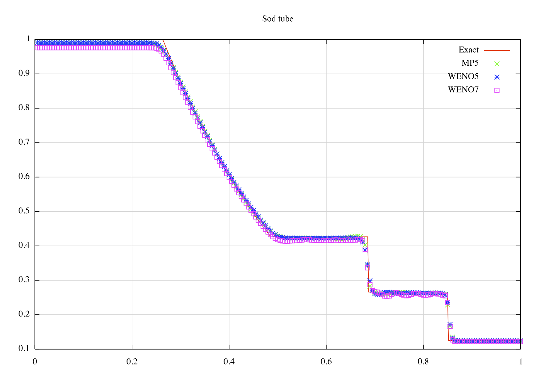
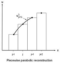
Yesterday I talked about a general purpose form for “limiters” applied to polynomial reconstructions, . For methods of this type the reconstruction is important because it defines the value of the function where there is not data, at cell-edges or faces where fluxes are computed, . For a method in conservation form the edge-face values are essential to updating the solution. As I will discuss the value of these values and mindful modifications of the values are severely under-utilized in implementing methods. Various methods can be improved in terms of accuracy, resolution, dissipation and stability through the techniques discussed in this post.

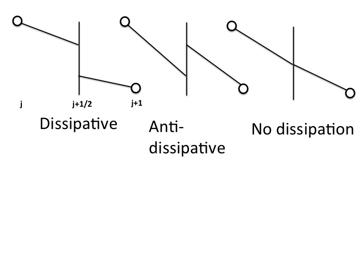
All of these techniques will utilize an important observation for methods of this type; one can swap edge-face values without impacting the accuracy of the method. Consider the reconstructed edge value that can (usually) be two values with a reconstruction being applied to $p\left(\theta_j \right)$ and $ p\left(\theta_{j+1} \right)$. If both reconstructions have equal accuracy we could trade these values, or replace one value by the other without impacting accuracy. Other properties like stability, dissipation or phase error are effected by this change, but formal accuracy is preserved.

One of the key aspects of the use of these edge values is a model for what an upwind method looks like applied to the data. Consider a nonlinear flux where upwinding will be applied to the edge values from two neighboring cells to determine the physically admissible flux, . An upwind approximation will use edge values from cells and . The simplest and most useful approximation of the flux is where is an eigen-decomposition of the flux Jacobian. The numerical dissipation is proportional to the eigenvalues and the jump at the cell edge . Generally speaking the physical direction of dissipation is defined by the jump from the cell-center (average) values, $latex– u_j $. The extrapolated edge values can (often) change the sign of the jump meaning that the approximation is locally anti-diffusive. A picture of faces is worth showing so one can understand what each swap looks like and envision the impact.

Perhaps the first application of this idea was the contact steepener defined by Colella and Woodward in their PPM method. Material interfaces also known as contact discontinuities are infamously diffused by Eulerian finite volume schemes even ones as high-resolution as PPM. The method introduced with PPM removes most of the diffusion usually induced by the method. The method works by locating valid interfaces and in the cells with the interface swapping the interface values at the edges. Often a material interface will be dissipative and swapping the edge values will be anti-diffusive. It is essential to apply a nonlinear stability mechanism to the swapped interface values and the polynomial reconstruction so that the anti-dissipative effects are not destabilizing. A second word of caution is the ill-advised nature of applying this technique at a nonlinear discontinuity such as a shock or rarefaction. For those flow features this technique would invite disaster.

A second, far safer application of edge swapping would be increasing the dissipation. In cases where the high-order local dissipation is anti-dissipative because the extrapolated values at the edges have a differently signed jump across the interface, swapping the edge values would make this dissipative. This condition has recently been dubbed as “entropy stable”. The condition can be computed by checking whether the jump in edge values has the same sign as the jump in cell-centered values . This should be particularly important in stably and physically moving nonlinear structures on the grid.  A concern is that too much dissipation is created as the figure shows. In this case the jump is entropy stable, but larger than the first-order method. This could actually be unstable especially if a Lax-Friedrichs flux is used because it is more dissipative than upwinding.

The penultimate approach would be to use these techniques to remove dissipation entirely from the edge. This is enabled by simply setting the two edge values to be equal in value. Any convex average of the edge values would achieve this as well as simply over-writing one of the edge values by the other. Like the anti-dissipative methods this would need to be applied with care for the stability of the overall integration procedure. In several cases the resulting approximation is actually higher order accurate. For example by applying this to first-order upwinding, the approximation is promoted to second-order central differencing. This happens for odd-ordered upstream centered methods, i.e., the third-order upwind methods is promoted to fourth-order centered edge values, the fifth-order upwind to sixth-order centered, and so forth.

The final approach to discuss would simply take one of the edge values and completely replace it by the other. The most obvious way to achieve this would be to declare that the information at the edge is unambigiously one-directional, and use that direction to choose the edge values. In this case one would short-circuit the Riemann solver and would only be stable for super-sonic flow. Of course, the opposite would produce a demonstrably anti-diffusive effect and might be useful (and dangerous too).

Don’t live a normal life by default, push the boundaries of your potential.

― Steven Redhead

Colella, Phillip, and Paul R. Woodward. “The piecewise parabolic method (PPM) for gas-dynamical simulations.” Journal of computational physics 54.1 (1984): 174-201.

Yang, Huanan. “An artificial compression method for ENO schemes: the slope modification method.” Journal of Computational Physics 89.1 (1990): 125-160.

Balsara, Dinshaw S., and Chi-Wang Shu. “Monotonicity preserving weighted essentially non-oscillatory schemes with increasingly high order of accuracy.”Journal of Computational Physics 160.2 (2000): 405-452.

Fjordholm, Ulrik S., Siddhartha Mishra, and Eitan Tadmor. “Arbitrarily high-order accurate entropy stable essentially nonoscillatory schemes for systems of conservation laws.” SIAM Journal on Numerical Analysis 50.2 (2012): 544-573.

Banks, Jeffrey William, and Jeffrey Alan Furst Hittinger. “A new class of nonlinear finite-volume methods for Vlasov simulation.” Plasma Science, IEEE Transactions on 38.9 (2010): 2198-2207.

Dumbser, Michael, and Olindo Zanotti. “Very high order P N P M schemes on unstructured meshes for the resistive relativistic MHD equations.” Journal of Computational Physics 228.18 (2009): 6991-7006.

Munz, Claus-Dieter, et al. “Enhanced Accuracy for Finite-Volume and Discontinuous Galerkin Schemes via Non-intrusive Corrections.” Recent Developments in the Numerics of Nonlinear Hyperbolic Conservation Laws. Springer Berlin Heidelberg, 2013. 267-282.

You can only exceed your limits if you’ve discovered them.

― Roel van Sleeuwen

About 15 years ago I wrote a simple paper with Len Margolin about options for modifying limiters used in high resolution schemes. Generally the paper didn’t get the success it deserved like so much else. It was studied by folks at Brown University, and was repurposed as a general positivity limiter. I will grant that the researchers at Brown did some really good work with the limiter especially proving how it could preserve accuracy (the positivity preserving limiter also preserves the design accuracy of the original reconstruction). I returned to this form in one of my recent papers, “Reconsidering Remap Methods” published earlier this year and the topic of a number of blog posts. Last week I realized that even more can be done with it and the form is really convenient for expressing a wide variety of nonlinear stability mechanisms in a more uniform manner.

The moment that crystalized my thinking was a re-reading and analysis of a limiter devised my Phil Colella and Michael Sekora for the PPM algorithm. This limiter was a “competitor” to an entirely different “limiting” strategy that I worked with Jeff Greenough and Jim Kamm. I now realized that the two limiters could be written in very nearly identical ways. Moreover, both of these ideas can be viewed as rather direct decedents of work by HT Huynh and Suresh from the late 1990’s. Each method attempts to extend nonlinear stability ideas beyond simply preserving monotonicity, to preserving valid extrema in solutions. Monontonicity preservation has the problem of seriously damping extrema with the limiter. All of these limiters can be expressed as different choices for a common form allowing direct comparison or mix and match ideas to be utilized effectively.

So, what is this common form?

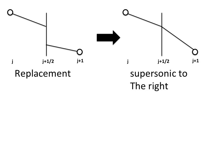
Given a polynomial (or more general functions perhaps) representation of a solution in a computational cell, where , the limiter is implemented as , is the general limiter and . The limiter has a general form, . The “Standard” is the test that defines the nonlinear control of the solution while “Reconstruction Choice” is the feature being controlled. I will give some examples below. It is important to note that is the reconstruction that produces an upwind scheme that is the canonical linear monotonicity preserving (positive) method, but only first-order accurate. Higher order polynomials can be defined for higher accuracy, but without the limiter they are invariably oscillatory.

The most common choice is the definition of a positivity preserving limiter. In this case where is the lowest value of that will be tolerated for physical reasons. Next our reconstruction is interrogated .

The same can be done for monotonicity-preserving limiters. Here the most common application is “slope-limiting” where a common choice is here is the famous minimum modulus function that returns the smallest magnitude argument if the arguments have the same sign. where is the “high-order” slope that you desire to use and control the stability of.

For extrema preservation I will provide a couple of choices from my own work and Colella & Sekora. In both cases the extrema preservation will only be applied if a local extrema is detected by the scheme. Generally speaking a monotonicity preserving limiter will help do this by setting .

The idea that I worked on had a couple of key concepts: don’t give up on the original high-order scheme yet, at an extrema a ENO or WENO scheme might be useful, and the monotonicity preserving method has good nonlinear stability properties. My limiter worked on edge values that then helped define the reconstruction polynomial. It turns out that the general limiter can work here too, , and everything else follows. The parts of the limiter are with being the monotonicity preserving edge value, is the high-order edge values and is the WENO edge value. Next, the limiter is completed with . Part of the key idea is to use two complimentary nonlinear stability properties from monotonicity preservation and WENO to assure the stability of the method should the high-order method be chosen. In this case the high-order method is bounded by two nonlinearly stable approximation choices. I thought it actually worked pretty well.

Colella and Sekora had a different approach based on looking at the local curvature (second derivative) of the parabolic reconstruction used in PPM. If the second derivatives of the reconstruction and the neighborhood of the reconstruction all have the same sign and roughly the same magnitude, the extrema is viewed as valid and worth propagating undistorted by the sort of damping monotonicity preserving methods produce. A simple way to implement this approach can be implemented using the general limiter I discuss. First we need to define the second derivative of the polynomial reconstruction . In this case the specifics of the limiter are where is the classical second derivative on the mesh and . The choice of method to define the denominator in the limiter is . The resulting limiter can either be applied to the edge values or equivalently to the reconstructing polynomial.

In my next post I will talk about how edge values, can be used productively to improve the robustness, resolution and stability of these methods.

Set Goals, not Limits.

― Manoj Vaz

Rider, William J., and Len G. Margolin. “Simple modifications of monotonicity-preserving limiter.” Journal of Computational Physics 174.1 (2001): 473-488.

Qiu, Jianxian, and Chi-Wang Shu. “A Comparison of Troubled-Cell Indicators for Runge–Kutta Discontinuous Galerkin Methods Using Weighted Essentially Nonoscillatory Limiters.” SIAM Journal on Scientific Computing 27.3 (2005): 995-1013.

Zhang, Xiangxiong, and Chi-Wang Shu. “Maximum-principle-satisfying and positivity-preserving high-order schemes for conservation laws: survey and new developments.” Proceedings of the Royal Society of London A: Mathematical, Physical and Engineering Sciences. The Royal Society, 2011.

Zhang, Xiangxiong, and Chi-Wang Shu. “On maximum-principle-satisfying high order schemes for scalar conservation laws.” Journal of Computational Physics229.9 (2010): 3091-3120.

Colella, Phillip, and Michael D. Sekora. “A limiter for PPM that preserves accuracy at smooth extrema.” Journal of Computational Physics 227.15 (2008): 7069-7076.

Suresh, A., and H. T. Huynh. “Accurate monotonicity-preserving schemes with Runge–Kutta time stepping.” Journal of Computational Physics 136.1 (1997): 83-99.

Huynh, Hung T. “Accurate upwind methods for the Euler equations.” SIAM Journal on Numerical Analysis 32.5 (1995): 1565-1619.

Rider, William J., Jeffrey A. Greenough, and James R. Kamm. “Accurate monotonicity-and extrema-preserving methods through adaptive nonlinear hybridizations.” Journal of Computational Physics 225.2 (2007): 1827-1848.