
TL;DR
In classical computational science applications for solving partial differential equations, discretization accuracy is essential. In a rational world, this solution accuracy would rule (other things are important too). It does not! Worse yet, the manner of considering accuracy is not connected to the objective reality of the method’s use. It is time for this to end. Two things influence true accuracy in practice. One is the construction of discretization algorithms, which have some counterproductive biases focused on order-of-accuracy. In real applications, solutions only achieve a low order of accuracy. Thus the accuracy is dominated by different considerations than assumed. It is time to get real.
“What’s measured improves” ― Peter Drucker
The Stakes Are Big
The topic of solving hyperbolic conservation laws has advanced tremendously during my lifetime. Today, we have powerful and accurate methods at our disposal to solve important societal problems. That said, problems and habits are limiting the advances. At the head of the list is a poor measurement of solution accuracy.
Solution accuracy is expected to be measured, but in practice only on ideal problems where full accuracy can be expected. When these methods are used practically, such accuracy cannot be expected. Any method will produce first-order or lower accuracy. Fortunately, analytical problems exist allowing accuracy to be assessed. The missing ingredient is to actually do the measurement. The benefit of changing our practice would cause focus energy and attention on methods that perform better under realistic circumstances. Today, methods with relatively poor accuracy and great cost are favored. This limits the power of these advances.
I’ll elaborate on the handful of issues hidden by the current practices. Our current dialog in methods is driven by high-order methods. These are studied without regard for their efficiency on real problems. The popular methods such as ENO, WENO, TENO, and discontinuous Galerkin dominate, but practical accuracy is ignored. A couple big issues I’ve written about reign broadly over the field. Time-stepping methods follow the same basic pattern. Inefficient methods with formal accuracy dominate over practical concerns and efficiency. We do not have a good understanding of what aspects of high-order methods pay off in practice. Some high-order aspects appear to matter, but others do not yield practical benefit. This includes truly bounding stability conditions for nonlinear systems, computing strong rarefactions-low Mach flows, and multiphysics integration.

The Bottom Line
I will get right to the punch line for my argument and hopefully show the importance of my perspective. Key to my argument is the observation that “real” or “practical” problems converge at a low order of accuracy. Usually, the order of accuracy is less than one, so assuming first-order accuracy is actually optimistic. The second key bit of assumption is what efficiency means in the context of modeling and simulation. I will define it as the relative cost of getting an answer of a specified accuracy. This seems obvious and more than reasonable.
“You have to be burning with an idea, or a problem, or a wrong that you want to right. If you’re not passionate enough from the start, you’ll never stick it out.” ― Steve Jobs

To illustrate my point I’ll construct a contrived simple example. Define three different methods to get our solution that are otherwise similar. Method 1 gives an accuracy of one for a cost of one. Method 2 gives an accuracy of twice as good as Method 1 for double the cost. Method 3 gives an accuracy of four times Method 1 and a cost of four times the cost. We can now compare the total cost for the same level of accuracy looking for the efficiency of the solution. Each method converges at the (optimistic) first-order rate.
If we use Method 3 on our “standard” mesh we get an answer with one-quarter the error for a cost of four. To get the same error as Method 2, we need to use a mesh of half the spacing (and twice the points). With Method 1 we need four times the mesh for the same accuracy. The relative cost of the equally accurate solution depends on the dimensionality of the problem. For transient fluid dynamics, we solve problems in one- two- or three-dimensions plus time. We are operating with methods that need to have the same time step control, the time step size is always proportional to the spatial mesh.
Let’s consider a one-dimensional problem, the cost scales quadratically with mesh (time and one space-time dimension). Our Method 2 will cost a factor of eight to get the same accuracy as Method 3. Thus is cost twice as much. Method 1 needs two mesh refinements for a cost of 16. Thus it costs four times as much as Method 3. So in one dimension, the more accurate method pays off tremendously, and this is the proverbial tip of the iceberg. As we shall see the efficiency gains grow in two or three dimensions.
In two dimensions the benefits grow. Now Method 2 costs 16 units and thus Method 3 pays off by a factor of four. For Method 1 we have a cost of 64 and the payoff is a factor of 16. You can probably see where this going. In three dimensions Method 2 now costs 32 and the payoff is a factor of 8. For Method 1 the payoff is huge. It now costs 256 times to get the same accuracy, Thus the efficiency payoff is a factor of 64. Almost two orders of magnitude difference. This is meaningful and important whether you are doing science or engineering.
Imagine how a seven-dimensional method like full radiation transport would scale. The payoffs for accuracy could be phenomenal. This is a type of efficiency that has been largely ignored in computational physics. It is time for it to end and focus on what really matters in computational performance. The accuracy under conditions actually faced in applications of the methods matters. This is real efficiency, and an efficiency not examined at all in practice.
“Progress isn’t made by early risers. It’s made by lazy men trying to find easier ways to do something.” ― Robert Heinlein

The Usual Approach To Accuracy
The usual approach to designing algorithms is to define basic “mesh” prototypically space and time. The usual mantra is that the most accurate methods are higher order. The higher order the method, the more accurate it is. High-order is often simply more than second-order accurate. Nonetheless, the assumption is that higher-order methods are always more accurate. Thus the best you can do is a spectral method. This belief has driven research in numerical methods forever (many decades at least). This is where every degree of freedom available contributes to the approximation. We know these methods are not practical for realistic problems.
The standard tool for designing methods is the Taylor series. This relies on several things to be true. The function needs to be smooth, and the expansion needs to be in a variable that is “small” in some vanishing sense. This is a classical tool and has been phenomenally useful for centuries of work in numerical analysis. The ideal nature of when it is true is also a limitation. While the Taylor series still holds for nonlinear cases, the dynamics of nonlinearity invariably destroy the smoothness. If smoothness is retained nonlinearly, the problem is pathological. The classic mechanism for this is shocks and other discontinuities. Even smooth nonlinear structures still have issues like cusps as seen in expansion waves. As we will discuss accuracy is not retained in the face of this.
If your solution is analytical in the best way possible this works. This means the solution can be differentiated infinitely. While this is ideal, it is also very infrequently (basically never) encountered in practice. The other issue is that the complexity of a method also grows massively as you go to a higher order. This is true for linear problems, but extra true for nonlinear problems where the error has many more terms. If it were only this simple! It is not by any stretch of the imagination.
“We must accept finite disappointment, but never lose infinite hope.” ― Martin Luther King Jr.
Stability: Linear and Nonlinear
For any integrator for partial differential equations, stability is a key property. Basically, it is a property where any “noise” in the solution decays away. The truth is that there is always a bit of noise in a computed solution. You never want it to dominate the solution. For convergent solution,s stability is one of two ingredients for convergence under mesh refinement. This is a requirement from the Lax equivalence theorem. The other requirement is the consistency of the approximation with the original differential equation. Together this yields the property of convergence where solutions become more accurate as meshes are refined. This principle is one of the foundational aspects of the use of high-performance computing.
Von Neumann invented a classical method to investigate stability. When devising a method, doing this analysis is a wise and necessary first step. Often subtle things can threaten stability and the method is good for unveiling such issues. For real problems, this stability is only the first step in the derivation. It is necessary, but not sufficient. Most problems have a structure that requires nonlinear stability.
This is caused by nonlinearities. in true problems or non-differentiable features in the solution (like shocks or other discontinuities. These require mechanisms to control things like oscillations and positivity of the solution. These mechanisms are invariably nonlinear even for linear problems. This has a huge influence on accuracy and the sort of accuracy that is important to measure. The nonlinear stability assures results in real circumstances. It has a relatively dominant impact on solutions and lets methods get accurate solutions when things are difficult. One of the damning observations is that the accuracy impact of these measures is largely ignored under realistic circumstances. The only thing really examined is robustness and low-level compliance with design.
“We don’t want to change. Every change is a menace to stability.” ― Aldous Huxley
What Accuracy Actually Matters
In the published literature it is common to see the accuracy reported for idealized conditions. These are conditions where the nonlinear stability is completely unnecessary. We do see if and how nonlinear stability impacts this ideal accuracy. This is not a bad thing at all. It goes into the pile of necessary steps for presenting a method. The problems are generally smooth and infinitely differentiable. A method of increasingly higher-order accuracy will get the full order of convergence and very small errors as the mesh is refined. It is a demonstration of the results of the stability analysis. This is to say that a stability analysis can provide convergence and error characterization. There is also a select set of problems for fully nonlinear effects (e.g., the isentropic vortex or the like).
“I have to go. I have a finite amount of life left and I don’t want to spend it arguing with you.” ― Jennifer Armintrout
There is a huge rub to this practice. This error and behavior for the method is never encountered in practical problems. For practical problems shocks, contacts, and other discontinuous phenomena abound. They are inescapable. Once these are present in the solution the convergence rate is first-order or less (theory for this exists). Now the nonlinear stability and accuracy character takes over being completely essential. The issue with the literature is that errors are rarely reported under these circumstances. This happens even if the exact error can be reported. The standard is simply “the eyeball norm”. This standard serves the use of these methods poorly indeed. Results under more realistic problems is close to purely qualitative. This happens even when there is an exact solution available.
One of the real effects of this difference comes down to the issue of what accuracy really matters. If the goal of computing a solution is to get a certain low level of error for the least effort, the difference is profound. The assessment of this might reasonably be called efficiency. In cases where the full order of accuracy can be achieved, the higher the order of the method, the more efficient it will be for small errors. These cases are virtually never encountered practically. The upshot is that accuracy is examined in cases that are trivial and unimportant.
Practical cases converge at first order and the theoretical order of accuracy for a method doesn’t change that. It can change the relative accuracy, but the relationship there is not one-to-one. That said, the higher order method will not always be better than a low order method. One of our gaps in analysis is understanding how the details of a method lead to practical accuracy. Right now, it is just explored empirically during testing. The issue is that the testing and reporting of said accuracy is quite uncommon in the literature. Making this a standard expectation would improve the field productively.
“Don’t be satisfied with stories, how things have gone with others. Unfold your own myth.” ― Rumi
References
Study of real accuracy
Greenough, J. A., and W. J. Rider. “A quantitative comparison of numerical methods for the compressible Euler equations: fifth-order WENO and piecewise-linear Godunov.” Journal of Computational Physics 196, no. 1 (2004): 259-281.
Nonlinear Stability
Guermond, Jean-Luc, and Bojan Popov. “Fast estimation from above of the maximum wave speed in the Riemann problem for the Euler equations.” Journal of Computational Physics321 (2016): 908-926.
Toro, Eleuterio F., Lucas O. Müller, and Annunziato Siviglia. “Bounds for wave speeds in the Riemann problem: direct theoretical estimates.” Computers & Fluids 209 (2020): 104640.
Li, Jiequan, and Zhifang Du. “A two-stage fourth order time-accurate discretization for Lax–Wendroff type flow solvers I. Hyperbolic conservation laws.” SIAM Journal on Scientific Computing 38, no. 5 (2016): A3046-A3069.
High Order Methods
Jiang, Guang-Shan, and Chi-Wang Shu. “Efficient implementation of weighted ENO schemes.” Journal of computational physics 126, no. 1 (1996): 202-228.
Cockburn, Bernardo, Chi-Wang Shu, Claes Johnson, Eitan Tadmor, and Chi-Wang Shu. Essentially non-oscillatory and weighted essentially non-oscillatory schemes for hyperbolic conservation laws. Springer Berlin Heidelberg, 1998.
Balsara, Dinshaw S., and Chi-Wang Shu. “Monotonicity preserving weighted essentially non-oscillatory schemes with increasingly high order of accuracy.” Journal of Computational Physics 160, no. 2 (2000): 405-452.
Cockburn, Bernardo, and Chi-Wang Shu. “Runge–Kutta discontinuous Galerkin methods for convection-dominated problems.” Journal of scientific computing 16 (2001): 173-261.
Spiteri, Raymond J., and Steven J. Ruuth. “A new class of optimal high-order strong-stability-preserving time discretization methods.” SIAM Journal on Numerical Analysis40, no. 2 (2002): 469-491.
Methods Advances Not Embraced Enough
Suresh, Ambady, and Hung T. Huynh. “Accurate monotonicity-preserving schemes with Runge–Kutta time stepping.” Journal of Computational Physics 136, no. 1 (1997): 83-99.
Colella, Phillip, and Michael D. Sekora. “A limiter for PPM that preserves accuracy at smooth extrema.” Journal of Computational Physics 227, no. 15 (2008): 7069-7076.
Rider, William J., Jeffrey A. Greenough, and James R. Kamm. “Accurate monotonicity-and extrema-preserving methods through adaptive nonlinear hybridizations.” Journal of Computational Physics 225, no. 2 (2007): 1827-1848.
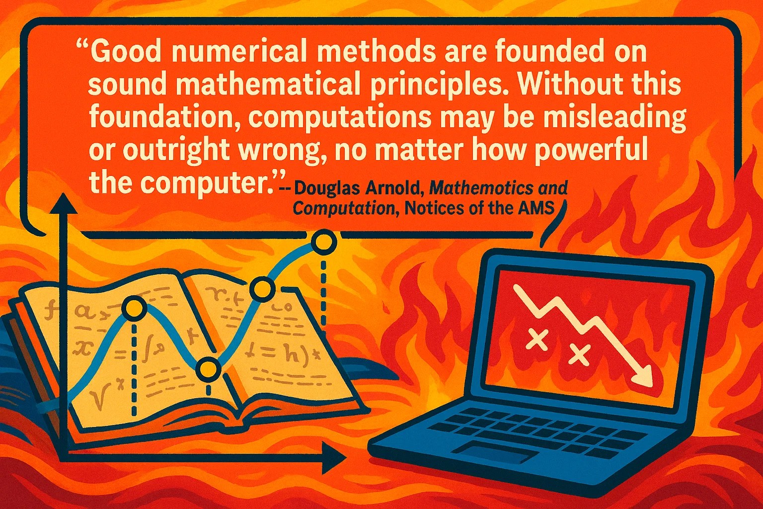

Pairing such a thoughtful discussion of the importance of accuracy with error-ridden AI images is pretty amusing. (AI image generators can always be relied on to produce exciting new words, such as mowerful, regarad, ehor, and mathemotics.)
Guilty as charged. I was playing with these for a splash of color. At least the prose was thoughtful
Absolutely! I always enjoy reading your insights.
This paper
Suresh, Ambady, and Hung T. Huynh. “Accurate monotonicity-preserving schemes with Runge–Kutta time stepping.” Journal of Computational Physics 136, no. 1 (1997): 83-99.
isn’t famous and not used as much as it should be because the authors are not in academia and not churning out a million variants of their approach unlike WENO.
and the following paper of yours is one of the first approaches I coded when I started learning CFD (shock capturing, etc) in 2016/17.
Rider, William J., Jeffrey A. Greenough, and James R. Kamm. “Accurate monotonicity-and extrema-preserving methods through adaptive nonlinear hybridizations.” Journal of Computational Physics 225, no. 2 (2007): 1827-1848.
P.S. Been reading your posts for a long time.
Thanks! Appreciate it!