tl;dr

If one goes back to the 1970s and 1980s, there was an explosion of activity around what became known as high-resolution methods. This was focused on overcoming Godunov’s Theorem, which limited linear monotone methods to being first-order. The key point was to introduce a mechanism, often called a limiter, that was a nonlinear switch between the first-order and the higher-order methods. This allowed both higher-than-first-order accuracy and the (approximate) monotonicity behavior, as desired. This sort of methodology was formalized with TVD methods introduced by Harten. TVD was a mathematical guide to nonlinearity in method composition. After this, high-resolution methods moved in a largely different direction with the idea of essentially non-oscillatory (ENO) methods. These methods discardedTVD. They were still based on monotone first-order methods. The issue is that ENO methods are inherently dissipative compared to the TVD methods for most practical problems. Their advantage on practical problems is only where highlydetailed structure and nonlinear things, such as turbulence or other phenomena, are present.

Here I introduce an idea for using TVD methods as a springboard to a new class of high-order accurate high-resolution methods. This will enable high accuracy of essentially non-oscillatory methods, matching TVD methods in situations where those are superior. This allows the higher accuracy results to meet the potential so often unmet in practice.

This is the first blog post written entirely after my retirement.

“Well, you want greater accuracy, but even more you want greater resolution. I defined a concept of resolution.” – Peter Lax

Prolog and Backstory

I’d like to start with a bit of personal background on this topic. The methods I’ll talk about are something that I thought about 20 years ago in my last months at Los Alamos. I’d even started to implement these methods in my personal research code. At that time, I had taken a management position, and my ability to execute any sort of deep technical work was highly compromised. Nonetheless, I started to look at these methods that I will describe below and implemented them in code. A combination of personal and professional reasons prompted me to move to Sandia. Then, while at Sandia, I completely subverted this interest to focus on the project work that I was hiredto do there. As is the way at Sandia, and I needed to fullycommit to that. Thus, these methods sat in the background for twenty years, not getting any attention. Much to my amazement, the ideas that I will describe here came rushing back to me as soon as I decided to retire. As soon as my mind was freed of all of the programmatic constraints at Sandia, I gave it the attention it deserved.

I think this episode says a lot about the intellectual environment at Sandia. In this specific area, Sandia’s methods and codes are so backwards that the ideas I will present here had no conceivable outlet. Sandia has serious problems with respect toinnovation and creation of new ideas. This is in spite of management declaring victory on this topic right before I left the lab. I can with some assurance state that the victory is hollow and not in evidence.

So, I hope you can enjoy this little aside into High Resolution Methods for hyperbolic PDEs.

Mathematical Foundations

“Well, when I started to work on it I was very much influenced by two papers. One was Eberhard Hopf’s on the viscous limit of Burgers’ equation, and the other was the von Neumann-Richtmyer paper on artificial viscosity. And looking at these examples I was able to see what the general theory might look like.” – Peter Lax

“My contribution to this point of view was that if you do that, then you have to set up a difference equation, which is in conservation form, which is consistent with the original conservation loss. That was a very useful observation.” – Peter Lax

If we go all the way to the beginning of the development of numerical methods, we can trace how we arrived here. The basic proof of concept was the first shock-capturing method using artificial viscosity. This stabilized and made practical an unstable method. Soon after, another type of method was produced, one that gave stable answers without this seemingly arbitrary stabilization. These were monotone methods that had naturally positive coefficients and suppressed oscillations by construction. Upwind methods are an archetype of this. Another introduced the conservation form and a different formulation in the Lax-Friedrichs method.

“Well, von Neumann saw the importance of stability and furthermore, he was able to analyze it. His analysis was rigorous for equation’s response to coefficients, linear analysis usually tells the story.” – Peter Lax

A canonical monotone scheme was Godunov’s method. This is basically extending upwind methods to systems of equations. This method alone would make Godunov legendary. Godunov also produced a seminal mathematical theorem. It is a barrier theorem telling us what cannot be done. It stated that a linear method could not be monotone as higher than first-order accuracy. All the original monotone methods are first order. Any second-order method is oscillatory. The keyword in this theorem is linear. Soon, a set of researchers would discover how to get past Godunov’s barrier theorem.

For approximations to hyperbolic PDEs, this spatial differencing is far and away the most important and influential aspect. This is not to discount or downplay the importance of dissipation mechanisms, Riemann solvers, or time differencing. Nonetheless, all of these are worthy of advancing, but none has the power to transform the field like the spatial approximation that’s used. This will play out over and over in this story.

A Revolution in Methods

“Well, you want greater accuracy, but even more you want greater resolution. I defined a concept of resolution.” – Peter Lax

It is clear that the key to overcoming Godunov’s barrier theorem was devised independently by four different researchers across the globe. Arguably, the first was Jay Boris, who devised flux limiters and the minmod function. Minmod returns the argument that is smallest in magnitude if the arguments all have the same sign. In this work, Jay produced a selection function that adapted fluxes to the nature of the solution. The key is that the approximation used depends on the solution. In other words, the approximation is nonlinear. This is the way out of Godunov’s barrier.

Bram Van Leer followed a similar path. Once I asked Bram, “How did you discover this?” Bram’s response was that he could just see that it could be done by examining plots of solutions from monotone methods and second-order schemes (canonically Lax-Wendroff). He could trace out the choices by eye, and he justneeded to come up with an automated mechanism. In the end, Van Leer came up with something quite similar toBoris. Ultimately, Van Leer produced a method that successfully updated Godunov’s method. Two other researchers, Ami Haren and Vladimir Kolgan, came up with their own nonlinear approximations.

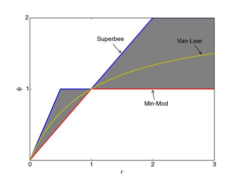
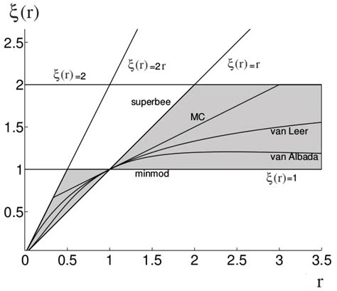
Ami Harten was an extraordinary mathematician and student of Peter Lax. In the 1980’s, he devised a way to formalize the advances in nonlinear approximations. This was the theory of total variation diminishing (TVD) methods. First-order monotone methods are TVD automatically. The TVD methods of second-order accuracy had weights that are nonlinear, and these weights came from limiters. He produced a theory that allowed one to determine if a limiter was suitable. This was formalized and graphically described by Sweby. The Sweby diagram has become canonical and inherently useful for examining methods.

These methods were a revelation for solving PDEs, particularly for fluid flow. Mathematicall,y these are known as hyperbolic equations (conservation laws). Suddenly, one did not have to choose between diffuse first-order solutions and non-physical oscillation rich higher order solutions. The difference in solution quality and efficiency was massiv,e especially in 2- or 3-D. The worst of these methods, using a minmod solution, was easily two to three times better than first-order Godunov on the Sod Shock tube. Sod’s shock tube is sort of a “Hello World” problem for shock waves. The better Van Leer method is over six times better (in 3-D this would be more than 100X.

These methods rapidly became state of the art in a host of communities across the technical World. This is most notable in Aerospace engineering, but also in astrophysics and nuclear weapons. These methods both benefited from the coattails of expanding computing power and the advent of CFD. The advance in accuracy offered by these methods was so great that it could not be ignored. It was a genuine quantum leap in performance. Now, second-order results could be found without oscillatory side-effects that were fatal for many applications. In some cases, calculations that had been impossible became physically attractive. Two great examples are turbulence and accretion discs.

Today, these methods are simply the standard and have not been replaced. There are good reasons for this!

The Development of ENO and Its Limitations

“The deepest sin against the human mind is to believe things without evidence. Science is simply common sense at its best – that is, rigidly accurate in observation, and merciless to fallacy in logic.” ― Thomas Huxley

The issue with TVD and similar methods are some distinct limits on what they can do. Mathematically, these methods are quite limited. The math itself is quite limited. These methods degenerate to first-order accuracy at any extrema in a solution. The theory does not extend cleanly to more than one dimension either. Thus, a gap exists between the desires of higher order accuracy and the observed practical utility of the methods. The practical utility drove rapid and widespread adoption. The lack of mathematical theory has provided a stagnation in progress.

Hyperbolic PDEs (and fluid dynamics) naturally produce singular structures like shocks or material interfaces. These structures inhibit high-order accuracy. For most practical applied uses of simulation, first-order accuracy and convergence are the best that can be expected. The theory for this is clear. Thus, high-order accuracy has limitations. This gets to the concept of high-resolution methods. The use of high-order accuracy increases the resolving power of the methods. The concept was first seen in a paper by Lax. This can most easily be seen in methods like PPM and generally in the work of Woodward and Colella. They use high-order methods as part of their otherwise “TVD” methods to get even better results.

The approach is to use methods higher than second-order as part of their second-order method. Unfortunately, their results are generally not built upon. Their work is simply seen as cornerstones and not foundations. I will try to place these in a more foundational position and show the way forward. We see this benefit in the quantum leap in accuracy and efficiency of these methods introduced to overcome Godunov’s theorem.

After the huge success of TVD methods, there was a distinct interest in continuing the revolution with new methods. Methods not limited in accuracy with more rigor were desired. One would think that the TVD methods would be the springboard to higher order as monotone methods had been. One attempt was made using TVB (total variation bounded methods. In this formulation, a constant is applied to TVD limiters to make the methods amenable to high-order accuracy. The issue is the constant, which becomes arbitrary and untethered to theory. The issue with TVB methods is the parameter, which does not have a good methodology for determining. It smacks of methods that have similar undetermined coefficients, like artificial viscosity. This approach rapidly lost favor and became a dead end. Below, I will suggest a different way to extend TVD to higher orders.

Before I get to that idea, let’s talk about the direction that did proceed. Essentially non-oscillatory methods were the path. The idea was to choose adaptively high-order approximations that were the least risky. Thereforethe approximation would always be high-order, but the safest approximation locally. This is simple in concept and had success, but major weaknesses too. Sometimes the approximations would be too unstable and lead to a breakdown. More often, the safety was overkill. These weaknesses led to the wildly popular weighted ENO (WENO) methods that introduced higher-order methods as the default fallback for approximation. Recently, Targeted ENO (TENO) has been introduced and has great appeal.

Nonetheles,s the penetration of these methods into practical problems has been quite dismal. If one looks at the Labs where I work, they have failed. Only the first generation of high-resolution methods (Van Leer’s) is used. There are very good reasons for this!

The issue with all these ENO methods is their resolving power. They all suck compared to TVD. They are only similar or less resolving than good TVD at a rather extreme cost. The actual practical resolution of ENO is closer to minmod TVD on simple or well-structured problems. So equivalent to the worst TVD method at an enormously higher cost. Getting formal high-order accuracy is not worth it. The only place these methods pay off are problems with a shitload of structure, like turbulence. Even though the payoff is modest. For practical problems, ENO is a dead end.

In the paper by Greenough and me about the accuracy of these methods. This is the impetus for developing different ideas as it showed ENO (WENO’s) limits and achilles heal.. This is the poor efficiency and payoff for complexity in practical results. one can have an answer just as bad as the worst TVD method for six times the cost. The core issue is that higher accuracy is incrediblyseductive. It is measured only on problems that nobody really cares about (the smooth ones). Thus, you have the notion of a third, fourth, fifth order method being available compared to a second-order method. The reality is that for problems you care about, the second-order method is actually more accurate and vastly more efficient. The practical utility is lost.

Other approaches to breaking out of this stagnation have also failed for a host of reasons. This includes discontinuous Galerkin (DG) methods that have great liabilities. Flux reconstruction is another approach that has failed to gain wide use. Some other methods have helped, such as MOOD or extremum-preserving methods (I worked on these too). None of them has caught fire and replaced TVD as the method of choice for real applications.

The Cure? The Median Function to the Rescue (Again!)

“The arc of our evolutionary history is long. But it bends towards goodness” ― Nicholas A. Christakis

For these practical problems with discontinuous solutions, the accuracy of the solution is rarely, if ever, measured. Thus, the entire issue discussed below is simply submerged. The community does not see it as accepted practice, and hence the problem does not get any attention. The starting point in digesting the results that I had in my paper with Jeff Greenough was to realize that the full non-linear WENO approach we studied was utilizedeverywhere on the grid. In actuality, for most places in the problem, it was completely unnecessary. The high-order approximation built into WENO was monotone all by itself. Thus, all of that effort in the WENO algorithm has no beneficial outcome. Actually, it is detrimental to accuracy.

This observation alone would comprise a new method with benefits. The recipe for the new method is quite simple to graft onto an existing ENO/WENO/TENO method. Given an existing or desired non-oscillatory method, the recipe is quite simple:

1. Take the ideal desired high-order method.

2. Test whether it is monotonicity preserving

3, If it is, then simply use the high-order method and exit

4. If it is not monotonicity preserving, use the ENO/WENO/TENO algorithm.

This is quite similar to Suresh and Huynh’s method, simply using a different approach at extrema or discontinuities. For what follows, this is the start of a more extensive modification. I will note that it is modestlymore accurate and efficient than the ENO/WENO?TENO method by virtue of NOT using those approximations everywhere. The monotonicity test is also quite simple and cheap to evaluate.

With this experience under my belt, I started to think about the creative arc that led to ENO. The original (OG as it were) monotone methods were first-order, but foundational for TVD methods. They were not replaced, but rather built on top of. The same methods are foundational for ENO. They are the low-order seed stencils that the high-order stencil is builtupon. Here is the key observation: with ENO, the TVD approximation is notbuilt upon. ENO goes back to the first-order approximation to create its higher-order approximation. What if we build high-order approximations using TVD as the low-order seed? What would this look like?

To me, this seemed a more logical progression for “ENO” type approximations. Rather than a first-order seed, we would begin with a second-order seed. This second-order seed for higher-order would be much more accurate than the first-order seed. The prospect is that the character of the TVD approximation would be transferredto the new high-order selection. This would cure the rather dismal practical accuracy problem that ENO/WENO/TENO methods are shackled by.

As the experienced reader of this blog might expect, I will use the $median\left(a,b,c\right)$ function to implement this. I love this function! This is an extension of the work of H. T. Huynh, who introduced and used this function in his work. Before unveiling my proposed methods, a bit of an aside is necessary. I will describe the median function and its known and potential properties. There are some significant keys to this function that makes its utility high.

1. $median\left(a,b,c\right)$ returns the argument that is bounded by the other two arguments. This argument is the convex combination of the other two. Hence, it is great for enforcing bounds if arguments have properties.

2. Accuracy is a proven property. If two of the three arguments are at least a certain order of accuracy, the function will return that order of accuracy. This comes from the median being a convex combination of those two arguments, or an argument that has that accuracy.

3. The first of my proposed properties is linear stability. This would be an extension of the accuracy property. This works under the premise of linearity, where the convex combination of stability would apply. This is almost certainly true.

4. Finally, the nonlinear stability is proposed as an outcome. This is the hardest to prove simply due to its nonlinearity. Nonlinear stability are things like total variation control or essential non-oscillatory behavior. It is not proven, but a hypothesis that seems quite reasonable and possible

Another key part of $median\left(a,b,c\right)$ is its connection to the essential minmod function. The $minmod\left(a,b\right)$ function was essential to TVD methods. It returns the minimum in absolute value between the arguments or zero if they differ in sign. There is an equivalence that is notable, $minmod\left(a,b\right) = median\left(a,b,0\right)$.In addition the minmod is usedin the simple implementation of median as $median\left(a,b,c\right) = a + minmod\left(b-a,c-a\right)$. I used the median function to express the PPM monotonicity limiter in what to me seemed an extremely clear manner.

The basic idea is use a standard TVD method as the base function for selecting a high-order approximation. This would include minmod, superbee, or Van Leer. One of the key premises is that the high-order method would inherit the character of the TVD base scheme. I will show how the method would be expressed for a new third-order method and then its natural extension, similar to the classic fifth-order WENO method.

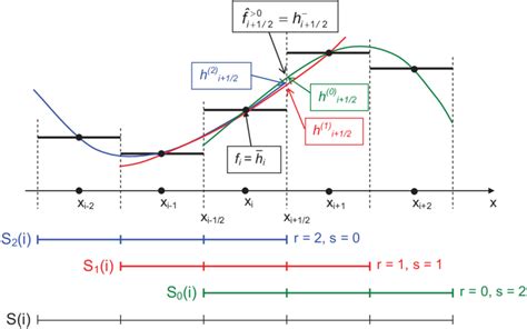
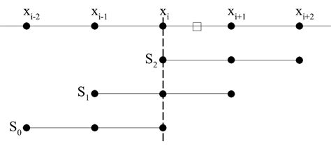
I will outline the algorithm proposed. Here are the basic elements of the method: $f_{TVD},$ the TVD approximation, $f_1$, $f_2$, and $f_3$, the third order methods with upstream bias, and $f_5$, the classic fifth orderupsteam centered method. The method for choosing a final method is then straightforward (the third-order method):

1. $f_a = median\left(f_{TVD}, f_1, f_2\right),$ $f_b = median\left(f_{TVD}, f_2, f_3\right)$.

2. $f_* = median\left(f_{TVD}, f_a, f_b\right).$

For discussion, we can see the approximation will be third-order accurate. One of the third-order methods is the classic ENO approximation with its weaker nonlinear stability property, thus that stability is inherited. Linear stability is far stronger as only one approximation in linearly unstable, and that property will be screened out.

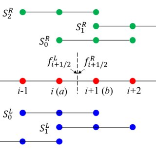
The fifth-order version is quite similar, with an extra step:

1. $f_a = median\left(f_{TVD}, f_1, f_2\right)$, $f_b = median\left(f_{TVD}, f_2, f_3\right)$.

2. $f_A = median\left(f_{TVD}, f_5, f_a\right), f_B = median\left(f_{TVD}, f_5, f_b\right).$

3. $f_* = median\left(f_{TVD}, f_A, f_B\right)$.

I have struggled to name this approach. My first idea was “nearly” TVD and then “almost” TVD. Neither is very technical nor mathematical sounding. Approximately TVD sounds better, but it doesn’t flow well. I have settled on “essentially” TVD or ETVD. The hope is that this approach comes closer to the desired design of ENO methods,$TV\left(u^{n+1}\right) \le TV\left(u^n\right) + \cal{O}\left(h^r\right)$. We note that the level of caution used in ENO has not served it well in terms of practical accuracy. This is thematically consistent with where methods have evolved.

This is a simple version of the proposed algorithm working on edge approximations that then become fluxes. A more proper version of the algorithm would measure the variation in a cell of the different approximations. This would be similar to or identical to the smoothness measures used in WENO. That variation would be usedto compare the results from different approximations. The complication from using this approach would be a post-processing step to find the proper edge value. One would find the variation that is closest to the TVD approximation. There are two obvious choices: one where a series of if-then statements finds the matching approximation. A second version would use the inverse variation measures to construct weights that would choose the approximation. These approaches use more data for the variation and weights. Testing would be required to determine the efficacy of the resulting method.

“In formal logic, a contradiction is the signal of a defeat; but in the evolution of real knowledge it marks the first step in progress towards a victory.” ― Alfred North Whitehead

Prospects Going Forward

In the not too distant futur,e I will show the results for these methods compared to ENO/WENO methods. This involves reanimating code from 20 years ago. The reanimated code will be greatly helped by some of the new AI coding tools. I had a very good experience compiling old code with OpenAI’s Codex. I may also try Claude Code. These tools are amazing. When I tried Codex it felt much like the amazement of using ChatGPT for the first time. Hopefully, I can compare the accuracy and efficiency of the methods using my old research code from my time at Los Alamos. I’m certain it will look appealing as my early tests showed, but I never really finalized or formalized my results before changing Labs.

“Keep in mind that there is in truth no central core theory of nonlinear partial differential equations, nor can there be. The sources of partial differential equations are so many – physical, probabilistic, geometric, etc. – that the subject is a confederation of diverse subareas, each studying different phenomena for different nonlinear partial differential equation by utterly different methods.”

– J Lindenstrauss, L C Evans, A Douady, A Shalev, and N Pippenge

References

Godunov, Sergei K., and Ihor Bohachevsky. “Finite difference method for numerical computation of discontinuous solutions of the equations of fluid dynamics.” Matematičeskij sbornik 47, no. 3 (1959): 271-306.

Lax, Peter D. “Hyperbolic systems of conservation laws II.” Communications on pure and applied mathematics 10, no. 4 (1957): 537-566.

Boris, Jay P., and David L. Book. “Flux-corrected transport. I. SHASTA, a fluid transport algorithm that works.” Journal of computational physics 11, no. 1 (1973): 38-69.

Van Leer, Bram. “Towards the ultimate conservative difference scheme. II. Monotonicity and conservation combined in a second-order scheme.” Journal of computational physics 14, no. 4 (1974): 361-370.

Van Leer, Bram. “Towards the ultimate conservative difference scheme. V. A second-order sequel to Godunov’s method.” Journal of computational Physics 32, no. 1 (1979): 101-136.

van Leer, Bram. “A historical oversight: Vladimir P. Kolgan and his high-resolution scheme.” Journal of Computational Physics230, no. 7 (2011): 2378-2383.

Lax, Peter D. “Accuracy and resolution in the computation of solutions of linear and nonlinear equations.” In Recent advances in numerical analysis, pp. 107-117. Academic Press, 1978.

Harten, Ami. “High resolution schemes for hyperbolic conservation laws.” Journal of computational physics 49, no. 3 (1983): 357-393.

Sweby, Peter K. “High resolution schemes using flux limiters for hyperbolic conservation laws.” SIAM journal on numerical analysis 21, no. 5 (1984): 995-1011.

Woodward, Paul, and Phillip Colella. “The numerical simulation of two-dimensional fluid flow with strong shocks.” Journal of computational physics 54, no. 1 (1984): 115-173.

Colella, Phillip, and Paul R. Woodward. “The piecewise parabolic method (PPM) for gas-dynamical simulations.” Journal of computational physics 54, no. 1 (1984): 174-201.

Colella, Phillip. “A direct Eulerian MUSCL scheme for gas dynamics.” SIAM Journal on Scientific and Statistical Computing 6, no. 1 (1985): 104-117.

Margolin, Len G., and William J. Rider. “A rationale for implicit turbulence modelling.” International Journal for Numerical Methods in Fluids 39, no. 9 (2002): 821-841.

Majda, Andrew, and Stanley Osher. “Propagation of error into regions of smoothness for accurate difference approximations to hyperbolic equations.” Communications on Pure and Applied Mathematics 30, no. 6 (1977): 671-705.

Banks, Jeffrey W., T. Aslam, and William J. Rider. “On sub-linear convergence for linearly degenerate waves in capturing schemes.” Journal of Computational Physics 227, no. 14 (2008): 6985-7002.

Shu, Chi-Wang. “TVB uniformly high-order schemes for conservation laws.” Mathematics of Computation 49, no. 179 (1987): 105-121.

Huynh, Hung T. “Accurate monotone cubic interpolation.” SIAM Journal on Numerical Analysis 30, no. 1 (1993): 57-100.

Huynh, Hung T. “Accurate upwind methods for the Euler equations.” SIAM Journal on Numerical Analysis 32, no. 5 (1995): 1565-1619.

Rider, William J., Jeffrey A. Greenough, and James R. Kamm. “Accurate monotonicity-and extrema-preserving methods through adaptive nonlinear hybridizations.” Journal of Computational Physics 225, no. 2 (2007): 1827-1848.

Suresh, Ambady, and Hung T. Huynh. “Accurate monotonicity-preserving schemes with Runge–Kutta time stepping.” Journal of Computational Physics 136, no. 1 (1997): 83-99.

Colella, Phillip, and Michael D. Sekora. “A limiter for PPM that preserves accuracy at smooth extrema.” Journal of Computational Physics 227, no. 15 (2008): 7069-7076.

Loubere, Raphaël, Michael Dumbser, and Steven Diot. “A new family of high order unstructured MOOD and ADER finite volume schemes for multidimensional systems of hyperbolic conservation laws.” Communications in Computational Physics 16, no. 3 (2014): 718-763.

Harten, Ami, and Stanley Osher. “Uniformly high-order accurate nonoscillatory schemes. I.” SIAM Journal on Numerical Analysis 24, no. 2 (1987): 279-309.

Harten, Ami, Bjorn Engquist, Stanley Osher, and Sukumar R. Chakravarthy. “Uniformly high order accurate essentially non-oscillatory schemes, III.” Journal of computational physics131, no. 1 (1997): 3-47.

Jiang, Guang-Shan, and Chi-Wang Shu. “Efficient implementation of weighted ENO schemes.” Journal of computational physics 126, no. 1 (1996): 202-228.

Fu, Lin. “Review of the High-Order TENO Schemes for Compressible Gas Dynamics and Turbulence.” Archives of Computational Methods in Engineering 30, no. 4 (2023).

Greenough, J. A., and W. J. Rider. “A quantitative comparison of numerical methods for the compressible Euler equations: fifth-order WENO and piecewise-linear Godunov.” Journal of Computational Physics 196, no. 1 (2004): 259-281.