This is my 400th post on the Regularized Singularity!

tl;dr

Few topics in computational physics are as polarizing as numerical dissipation. Dissipation is ubiquitous in nature and technology. Often, it is unwanted or a nuisance. Its absence is usually wishful thinking. Some schools of thought think they can model it effectively. For general numerical modeling, some sort of effective dissipation is essential to robust, reliable simulations. To understand the various viewpoints requires a far more nuanced perspective. Numerical dissipation or its absence is the direct result of different philosophies. Usually, the grounding philosophy is unstated and implicit. Here we explore this in depth.

“Whenever a theory appears to you as the only possible one, take this as a sign that you have neither understood the theory nor the problem which it was intended to solve.” ― Karl Popper

The Physics of Dissipation

The physics of dissipation is essential. The part of dissipation that is least important in current methodology is that which is well resolved. I mean no disrespect towards the types of physics appearing at the nano scale or in well-resolved areas with very exotic viscoelastic effects. The really important parts for nature and technology are where the dissipation is so small it can’t be resolved. These are challenging in the extreme. The truth is that there is a certain magic in dissipation at those scales, where the amount of energy and entropy evolve due to the non-linear impact of the hyperbolic parts of the system. These dynamics remain mysterious.

This sort of physics dominates shock waves and turbulence. If one is dealing with highly energetic physics of almost any kind in technology or nature, one is dealing with these sorts of physics. Moreover, detailed direct numerical simulation of this kind of physics is a pipe dream, and there’s no way that computers available in any of our lifetimes will be able to tackle this. It is completely out of scope. It is also the kind of physics where AI isn’t the way out. It requires deep understanding and mathematics that is often quite just beyond our reach. We need a focused exploration of the physics and mathematics of it. Something we are not doing as a society.

This is exactly the domain where numerical dissipation is essential for computational science, and all the controversy lives. There are two main schools of thought:

1. This is built into the dissipation to the numerics, effectively making it implicit or modeling it. The domain of Riemann solvers and high-resolution methods.

2. One of the more foolhardy aspects is that the physical modeling that we have today is actually up to the task of accurately depicting its effects.

The thing that’s often missing is an understanding of how numerical techniques like artificial viscosity are intimately related to the fundamental models. They are far more the same than different, and there lies the path ahead.

“In theory, there is no difference between theory and practice. But in practice, there is.” ― Benjamin Brewster

Shock Capturing and Dissipation

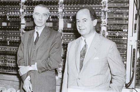
To understand numerical dissipation, its origins are essential. Artificial viscosity allowed shock-capturing methods to work, but I need to rewind a little. In World War 2 the USA built an atomic bomb. Part of the design and creation of the weapon was numerical simulations of shock waves. This was, to a large degree, the vision of John Von Neumann. It was brought to life in Los Alamos by Feynman and Bethe. Von Neumann had developed a numerical method for solving shock waves. The issue was that it failed spectacularly ( blowing up into horrible oscillations). I

Instead, a method designed by a cadre of the British mission developed a method that worked. Peierls and Skryme worked on ideas using shock tracking plus finite difference (well documented by Morgan and Archer). This method successfully computed the problem they set before them. They also puzzled over the failure of Von Neumann’s method. Peierls suggested that dissipation was the missing element, but the greats of Los Alamos moved on. After the war, as the Cold War was warming up, Robert Richtmyer returned to this problem. The work at Los Alamos had grown in complexity, and the methods of WW2 weren’t up to the task.

In 1947 and 1948, Richtmyer devised a numerical dissipation to add to Von Neumann’s method. It worked extremely well and was published to the World by him and Von Neumann in 1950. This method was called artificial viscosity. The derivation by Richtmyer was based on the physics of shock waves and the changes in entropy required for the correct solution. These asymptotics were embedded in the method, and Richymer’s method was not arbitrary. This method was then a proof of principle.

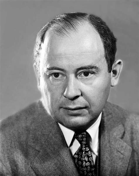
In short order, the use of dissipation made methods work, and many methods flourished. Harlow at Los Alamos could advance new ideas for methods and codes. Lax was inspired by Los Alamos and created a method where dissipation was implicit in the differencing method. There was no added viscosity. Instead, the viscosity was built into his Lax-Friedrichs method. Von Neumann took his ideas to Princeton (and the Institute for Advanced Study). There, he was interested in weather (and climate) modeling.

“It doesn’t matter how beautiful your theory is, it doesn’t matter how smart you are. If it doesn’t agree with experiment, it’s wrong.” ― Richard P. Feynman

In 1956, Norm Phillips did the initial calculations of a month of weather in the Eastern USA. All was well except for the appearance of those pesky oscillations by the end of the month. The follow-on work fell to Joseph Smagorinsky (that name should be familiar). Smagorinsky was going to move to 3-D and implement a suggestion to fix the oscillations (ringing). The suggestion was made by Von Neumann’s famous collaborator, Jules Charney. The work culminated with his 1963 paper, which was simultaneously the first LES calculation and global circulation model. The artificial viscosity was implemented, too. This was the first LES model, and it was just a trivial (naive) 3-D implementation.

Thus, the first LES model was simply Von Neumann-Richtmyer artificial viscosity!

This gets used to model as an alternative to numerical viscosity, implicit or explicit. It would be too much to call it bullshit to model it, but not by much. Modeling is a completely desirable and valid activity. The wrong thing is failing to see the basis of this effective model. There are some clear messages that we’ve failed to take. How is a method based on shock dynamics also an effective turbulence model? How much of the model is physics, and how much is numerical stability? Are the two concepts remotely separable?

Modeling and Dissipation

“It is the theory which decides what can be observed” ― Albert Einstein

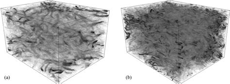
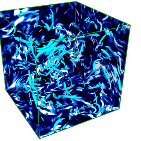
The place where all of this collides most acutely is turbulence modeling. Turbulence modeling has three basic flavors: direct numerical simulation (DNS), large eddy simulation (LES), and Reynolds-averaged Navier-Stokes (RANS). These each come with limits and capabilities. By the same token, the state of the art is still lacking. I think the reasons for this flow through this topic.

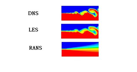
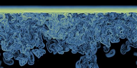
Let us start with DNS. It is a useful practice where no model is used at all, other than the Navier-Stokes equations. The numerical solution is just an accurate method solved with a fine mesh. The resolution is largely a rule of thumb and common practice. Numerical error is rarely or never estimated. The solutions compute and don’t look like shit, and they are accepted. DNS is very limited. We struggle to compute “hard turbulence” with our biggest computers. The scaling with computing power is quite dismal as well.

Worse yet, it is canonically incompressible. I’ve noted that incompressibility is grossly unphysical in several respects. The largest issue is causality, where the sound speed is infinite, and thermodynamics is annihilated. Thus, this part of the simulation is divorced from the physics that could be the heart of the solution. I believe it is very likely that the solution to turbulence theory may well be found with thermodynamics and shock wave dynamics.. This would be in the opposite asymptotic regime to where it is usually focused on.

LES comes next, allowing more to be done. As noted, the classical model is the Smagorinsky dissipation, which in turn is just artificial viscosity. Its simple and naive form is its Achilles heel. There are none of the structural changes embedded in it that have been added to artificial viscosity. For example, artificial viscosity is turned off in adiabatic regions. These differences correlate strongly with the modeling suggested by scale similarity models. The origin of LES should be recognized along with all the aspects missed when the two uses are separated. There has never been a reintegration of the topic after its birth. Perhaps implicit LES (ILES) is a sort of this.

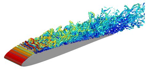
Finally, we have modeling with RANS. It comes with modeling approaches starting with simple eddy viscosity models all the way to very elaborate moment closures. These models are supposed to look at statistical ensembles of flows averaged in some manner. The models are designed to capture the average behavior of flows. In general, these are essential to the engineered application of systems. Typically, these have issues and requirements for things like boundary layers, where numerical resolution is demanding. They are also integrated by methods that usually have a great deal of implicit built-in dissipation.

This is our next stop.

“There is only one kind of shock worse than the totally unexpected: the expected for which one has refused to prepare.” ― Mary Renault

Implicit Dissipation

“Any sufficiently advanced technology is indistinguishable from magic.” – Arthur C. Clarke

Now we turn to the built-in dissipation of methods. I touched on this with the work of Lax. The canonical method with implicit dissipation is upwind differencing. This method is most cleanly and broadly described by Godunov’s method, where the Riemann problem is employed to determine the upwind propagation. In many quarters, upwind differencing and dissipation are treated with absolute disdain and ridicule.

As I found in my work on ILES, the issue with upwind methods is the order of accuracy. The ridicule should be confined to the first-order version of the method. We discovered that the combination of second-order accuracy and conservation form yielded a different conclusion. This combination converts the truncation error for quadratic nonlinearities to something “magical”. The form of the nonlinear error changes energy and responds to the physics of the flow. The form in 3-D conforms to the scale similarity model from LES. If one then adds selective dissipation via upwind (Riemann solvers), the method acts like a smart LES model. This recipe of techniques is present in most ILES examples. It is relatively obvious that it is the core of the success that many turbulence researchers find so annoying.

As I have and will write, the modern methods have serious gaps and issues. I recently wrote about issues around evolving adiabatic flows. The methods have a host of pathologies, mostly known due to their broad and extensive use. High-order and high-resolution are still being sorted out. The ultimate efficiency and effectiveness of the methods are still being worked on. The field requires new directions and breakthroughs. Still, these methods have an amazing track record of success, and they are key bits of modern computational technology.

“The essence of science is that it is always willing to abandon a given idea for a better one; the essence of theology is that it holds its truths to be eternal and immutable.” ― H.L. Mencken

References

VonNeumann, John, and Robert D. Richtmyer. “A method for the numerical calculation of hydrodynamic shocks.” Journal of applied physics 21, no. 3 (1950): 232-237.

Margolin, Len G., and K. L. Van Buren. “Richtmyer on Shocks:“Proposed Numerical Method for Calculation of Shocks,” an Annotation of LA-671.” Fusion Science and Technology 80, no. sup1 (2024): S168-S185.

Mattsson, Ann E., and William J. Rider. “Artificial viscosity: back to the basics.” International Journal for Numerical Methods in Fluids 77, no. 7 (2015): 400-417.

Morgan, Nathaniel R., and Billy J. Archer. “On the origins of Lagrangian hydrodynamic methods.” Nuclear Technology 207, no. sup1 (2021): S147-S175.

Lax, Peter D. “Hyperbolic systems of conservation laws II.” Communications on pure and applied mathematics 10, no. 4 (1957): 537-566.

Harlow, Francis H. “Fluid dynamics in group T-3 Los Alamos national laboratory:(LA-UR-03-3852).” Journal of Computational Physics 195, no. 2 (2004): 414-433.

Smagorinsky, Joseph. “General circulation experiments with the primitive equations: I. The basic experiment.” Monthly weather review 91, no. 3 (1963): 99-164.

Smagorjnsky, Joseph. “The beginnings of numerical weather prediction and general circulation modeling: early recollections.” In Advances in geophysics, vol. 25, pp. 3-37. Elsevier, 1983.

Grinstein, Fernando F., Len G. Margolin, and William J. Rider, eds. Implicit large eddy simulation. Vol. 10. Cambridge: Cambridge university press, 2007.

Godunov, Sergei K., and Ihor Bohachevsky. “Finite difference method for numerical computation of discontinuous solutions of the equations of fluid dynamics.” Matematičeskij sbornik 47, no. 3 (1959): 271-306.

Margolin, Len G., and William J. Rider. “A rationale for implicit turbulence modelling.” International Journal for Numerical Methods in Fluids 39, no. 9 (2002): 821-841.