Divide each difficulty into as many parts as is feasible and necessary to resolve it.

― René Descartes

In numerical methods for partial (integral too) differential equations there are two major routes to solving problems “well”. One is resolving the solution (physics) with some combination of accuracy and discrete degrees of freedom. This is the path of brute force where much of the impetus to build ultra-massive computers comes from. It is the tool of pure scientific utilization of computing. The second path is capturing the physics where ingenious methods allow important aspects of the solution to be found without every detail being known. This methodology forms the backbone of and enables most useful applications of computational modeling. Shock capturing is the archetype of this approach where the actual singular shock is smeared (projected) onto the macroscopic grid instead of demanding infinite resolution through the application of a carefully chosen dissipative term.

In reality both approaches are almost always used in modeling, but their differences are essential to recognize. In many of these cases we resolve unique features in a model such as the geometric influence on the result while capturing more universal features like shocks or turbulence. In practice, modelers are rarely so intentional about this or what aspect of numerical modeling practice is governing their solutions. If they were the practice of numerical modeling would be so much better. Notions of accuracy, fidelity and general intentionality in modeling would improve greatly. Unfortunately we appear to be on a path to allow an almost intentional “dumbing down” of numerical modeling by dulling down the level knowledge associated with the details of how solutions are achieved. This is the black box mentality that dominates modeling and simulation in the realm of applications.

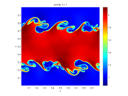
No where does the notion of resolving physics come into play like direct numerical simulation of turbulence, or direct simulation of any other physics for that matter. Turbulence is the archetype of this approach. It also serves are a warning to anyone interested in attempting this approach. In DNS there is a conflict between fully resolving the physics and most successfully computing the most dynamic physics given existing computing resources. As a result the physics being computed by DNS rarely uses a mesh in the “asymptotic” range of convergence. Despite being fully resolved, DNS is rarely if ever subjected to numerical error estimation. In the cases where this has been achieved the accuracy of DNS falls short of expectations for “resolved” physics. In all likelihood truly resolving the physics would require far more refined meshes than current practice dictates, and would undermine the depth of scientific exploration (lower Reynolds numbers). We see the balance between quality and exploration in science is indeed a tension that remains ironically unresolved.

Perhaps more concerning is the tendency to only measure the integral response of systems subject to DNS. We rarely see a specific verification of the details of the small scales that are being resolved. Without all the explicit and implicit work to assure the full resolution of the physics, one might be right to doubt the whole DNS enterprise and its results. It remains a powerful tool for science and a massive driver for computing, but due diligence on its veracity remains a sustained shortcoming in its execution. As such the greater degree of faith in DNS results should be an endeavor of science rather than simply granted by fiat, as we tend to do today.

Given the issues with fully resolving physics where does “capturing” fit? In principle capturing means that the numerical method contains a model that allows it to function properly when the physics is not resolved. It usually means that the method will reliably produce integral properties of the solution. This is achieved by building the right asymptotic properties into the method. The first and still archetypical method is shock capturing and artificial viscosity. The method was developed to marry a shock wave to a grid by smearing it across a small number of mesh cells and adding the inherent entropy production to a method. Closely related to this methodology is large eddy simulation, which allows under-resolved turbulence to be computed. The subgrid model in its simplest form is exactly artificial viscosity from the first shock capturing method, and allows the flow to dissipate at a large scale without computing the small scales. It also stabilizes what would otherwise be an unstable computation.

Another major class of physics capturing is interface or shock tracking. Here a discontinuity is tracked with the presumption that it is a sharp transition between two states. These states could be the interface between two materials, or pre- and post-shock values. In any cases a number of assumptions are encoded into the method on the evolution of the interface and how the states change. Included are rules for the representation of the solution, which define the method’s performance. Of course, stability of the method is of immense importance and the assumptions made in the solution can have unforeseen side-effects.

One of the key issues for the pragmatic issues associated with the resolved versus captured solution is that most modern methods blend the two concepts. It is a best of both Worlds strategy. Great examples exist in the World of high-order shock capturing methods. Once a shock exists all of rigor in producing high-order accuracy becomes a serious expense compared to the gains in accuracy. The case for using higher than second order method remains weak to this day. The question to be answered more proactively by the community is “how can high-order methods be used productively and efficiently in production codes?”

Combining the concepts of resolving and capturing is often done without any real thought on how this impacts issues of accuracy, and modeling. The desire is to have the convenience-stability-robustness of capturing with the accuracy associated with efficient resolution. Achieving this for anything practical is exceedingly difficult. A deep secondary issue is the modeling inherent in capturing physics. The capturing methodology is almost always associated with embedding a model into the method. People will then unthinkingly model the same physical mechanisms again resulting in a destructive double counting of physical effects. This can confound any attempt to systematically improve models. The key question to ask about the solution, “is this feature being resolved? Or is this feature being captured?” The demands on the computed solution based on the answer to these simple questions are far different.

These distinctions and differences all become critical when the job of assessing the credibility of computational models. Both the modeling aspects, numerical error aspects along with the overall physical representation philosophy (i.e., meshing) become critical in defining the credibility of a model. Too often those using computer codes to conduct modeling in scientific or engineering contexts are completely naïve and oblivious to the subtleties discussed here.

In many cases they are encouraged to be as oblivious as possible about many of the details important in numerical modeling. In those cases the ability to graft any understanding onto the dynamics of the numerical solution of the governing equations onto their analysis becomes futile. This is common when the computer code solving the model is viewed as being a turnkey, black box sort of model. Customers accepting results presented in this fashion should be inherently suspicious of the quality. Of course, the customers are often encouraged to be even more naïve and nearly clueless about any of the technical issues discussed above.

Resolve, and thou art free.

― Henry Wadsworth Longfellow

Our greatest fear should not be of failure but of succeeding at things in life that don’t really matter.

― Francis Chan

Vacations are a necessary disconnection from the drive and drain of the every day events of our lives. They are also necessary to provide perspective on things that become to commonplace within the day in day out. My recent little vacation was no different. I loved both Germany and France, but came to appreciate the USA more too. Europeans and particularly Parisians smoke in tremendous numbers. It makes a beautiful city like Paris a bit less ideal and uncomfortable. My wife has recently had major surgery that limits her mobility, and European accommodation for disabilities and handicaps are terrible in comparison to the USA.   

So the lesson to be learned is that despite many issues, the USA is still a great place and better than Europe in some very real ways. These interesting observations are not the topic here, which is another observation born of vacation time and its numerous benefits.

Bureaucracy destroys initiative. There is little that bureaucrats hate more than innovation, especially innovation that produces better results than the old routines. Improvements always make those at the top of the heap look inept. Who enjoys appearing inept?

― Frank Herbert

Another thing I noted was the irritation I feel when formality trumps substance in work. Formality has its place, but when it stifles initiative, innovation and quality, it does more harm than good. There was an activity at work that I had finished prior to leaving. Anything related to the actual work of it was utterly complete. It involved reviewing some work and denoting whether they had completed the work promised (it was in our parlance, a milestone). They had, and in keeping with current practice for such things, the bar was set so low that they would have had an almost impossible time not succeeding. Despite the relative lack of substance to the entire affair, the old fashioned memo to management was missing (the new fashioned memo with electronic signature was finished, and delivered). Here form was subservient to function and effort was expended in a completely meaningless way.

I had committed to taking a real vacation; I was not going to waste Paris doing useless administrative work. I screened my e-mail and told the parties involved that I would deal with it upon my return. Yet people wouldn’t let go of this. They had to have this memo signed in the old-fashioned way. In the end I thought what if they had put as much effort into doing old-fashioned work? What of instead of dumbing down and making the work meaningless to make sure of success, the work had been reaching far, and focused on extending the state of practice? Well then it might have been worth a bit of extra effort, but the way we do work today, this administrative flourish was simply insult to injury.

Management cares about only one thing. Paperwork. They will forgive almost anything else – cost overruns, gross incompetence, criminal indictments – as long as the paperwork’s filled out properly. And in on time.

― Connie Willis

The experience makes it clear, today we value form over function, appearances over substance. It is an apt metaphor for how things work today. We’d rather be successful doing using useless work than unsuccessful doing useful work. A pathetic success is more valuable than a noble failure. Any failure is something that induces deep and unrelenting fear. The inability to fail is hampering success of the broader enterprise to such a great degree as to threaten the quality of the entire institution (i.e., the National Lab system).

The issue of how to achieve the formality and process desired without destroying the essence of the Lab’s excellence has not been solved. Perhaps if credit were given for innovative, risk-taking work so that the inevitable failures were not penalized would be a worthy start. In terms of impact on all the good that the Labs do, the loss of the engines of discovery they represent negatively impacts national security, the economy, the environment and the general state of human knowledge. Reversing these impacts and puts the Labs firmly in the positive column would be a monumental improvement.

It is hard to fail, but it is worse never to have tried to succeed.

― Theodore Roosevelt

The epitomes of these pathetic successes are milestones. Milestones measure our programs, and seemingly the milestones denote important, critical work. Instead of driving accomplishments, the milestones sew the seeds of failure. This is not specifically recognized failure, but the failure driven by the long-term decay of innovative, aggressive technical work. The reason is the view that milestones cannot fail for any reason, and this knowledge drives any and all risk from the definition of the work. People simply will not take a chance on anything if it is associated with a milestone. If we are to achieve excellence this tendency must be reversed. Somehow we need to reward the taking of risks to power great achievements. We are poorer as a society for allowing the current mindset to become the standard.

Without risk, we systematically accomplish less innovative important work, and ironically package the accomplishment of relatively pathetic activities as success. To insure success, good work is rendered pathetic so that the risk of failure is completely removed. It happens all the time, over and over. It is so completely engrained into the system that people don’t even realize what they are doing. To make matters worse, milestones command significant resources be committed toward their completion. So we have a multitude of sins revolving around milestones: lots of money going to execute low-risk research masquerading as important work.

Over time these milestones come to define the entire body of work. This approach to managing the work at the Labs is utterly corrosive and has aided the destruction of the Labs as paragons of technical excellence. We would be so much better off if a large majority of our milestone failed, and failed because they were so technically aggressive. Instead all our milestones succeed because the technical work is chosen to be easy. Reversing this trend requires some degree of sophisticated thinking about success. In a sense providing a benefit for conscientious risk-taking could help. We still could rely upon the current risk-averse thinking to provide systematic fallback positions, but we would avoid making the safe, low-risk path the default chosen path.

Only those who dare to fail greatly can ever achieve greatly.

― Robert F. Kennedy

One place where formality and substance collide constantly is the world of V&V. The conduct of V&V is replete with formality and I generally hate it. We have numerous frameworks and guides that define how it should be conducted. Doing V&V is complex and deep, never being fully defined or complete. Writing down the process for V&V is important simply for the primary need to grapple with the broader boundaries of what is needed. It is work that I do, and continue to do, but following a framework or guide isn’t the essence of what is needed to do V&V. An honest and forward-looking quality mindset is what V&V is about.

It is a commitment to understanding, curiosity and quality of work. All of these things are distinctly lacking in our current culture of formality over substance. People can cross all the t’s and dot all the i’s, yet completely failed to do a good job. Increasingly the good work is being replaced by formality of execution without the “soul” of quality. This is what I see, lots of lip service paid to completion of work within the letter of the law, and very little attention to a spirit of excellence. We have created a system that embraces formality instead of excellence as the essence of professionalism. Instead excellence should remain the central tenet in our professional work with formality providing structure, but not the measure of it.

Bureaucracies force us to practice nonsense. And if you rehearse nonsense, you may one day find yourself the victim of it.

― Laurence Gonzales

Let’s see how this works in practice within V&V, and where a different perspective and commitment would yield radically different results.

I believe that V&V should first and foremost be cast as the determination of uncertainties in modeling and simulation (and necessarily experimentation as the basis for validation). Other voices speak to the need to define the credibility of the modeling and simulation enterprise, which is an important qualitative setting for V&V work. Both activities combine to provide a deep expression of commitment to excellence and due diligence that should provide a foundation for quality work.

I feel that uncertainties are the correct centering of the work in a scientific context. These uncertainties should always be quantitatively defined, that is should never be ZERO, but always have a finite value. V&V should push people to make concrete quantitative estimates of uncertainty based on technical evidence accumulated through focused work. Sometimes this technical evidence is nothing more than expert judgment or accumulated experience, but most of time much more. The true nature of what is seen in work done today whether purely within the confines of customer work or research shown at conferences or in journals does not meet these principles. The failure to meet these principles isn’t a small quibbling amount, but a profound systematic failure. The failure isn’t really a broad moral problem, but a consequence of fundamental human nature at work. Good work does not provide a systematic benefit and in many cases actually provides a measurable harm to those conducting it.

Today, many major sources of uncertainty in the modeling, simulation or experimentation are unidentified, unstudied and systematically reported as being identically ZERO. Often this value of ZERO is simply implicit. This means that the work doesn’t state that it’s “ZERO,” but rather fails to examine the uncertainties at all leading to it being a nonentity. In other words the benefit of doing no work at all is reporting a smaller uncertainty. The nature of the true uncertainty is invisible. This is a recipe for an absolute disaster.

A basic principle is that doing more work should result in smaller uncertainties. This is like a statistical sampling where gathering more samples systematically produces a smaller statistical error (look at standard error in frequentist statistics). The same thing applies to modeling or numerical uncertainty. Doing more work should always reduce uncertainties, but the uncertainty is always finite, and never identically ZERO. Instead by doing no work at all, we allow people to report ZERO as the uncertainty. Doing more work can only result in increasing the uncertainty. If doing more work increases the uncertainty the proper conclusion is that your initial uncertainty estimate was too small. The current state of affairs is a huge problem that undermines progress.

Here is a very common example of how it manifests itself in practice. The vast majority of computations for all purposes do nothing to estimate numerical errors, and get away with reporting an effective value of ZERO for the numerical uncertainty. Instead of ZERO if you have done little or nothing to structurally estimate uncertainties, your estimates should be larger than the truth to account for your lack of knowledge. Less knowledge should never be rewarded with reporting smaller uncertainty.

For example you do some work and find out that the numerical uncertainty is larger than your original effort. The consequence is that your original estimate was too small and you should learn about how to avoid this problem in the future. Next time doing more work and getting to report a smaller uncertainty should then reward you. You should also do the mea culpa and admit that your original estimate was overly optimistic. Remember V&V is really about being honest about the limitations of modeling and simulation. Too often people get hung up on being able to do complete technical assessment before reporting any uncertainty. If the full technical work cannot be executed, they end up presenting nothing at all, or ZERO.

People get away with not doing numerical error estimation in some funny ways. Here is an example that starts with the creation of the numerical model for a problem. If the model is created so that it uses all the reasonably available computing resources, it can avoid estimating numerical errors by a couple of ways. Often these models are created with an emphasis of computational geometric resolution. Elements of the problem are meshed using computational elements that are one thick (or wide or tall). As a result the model cannot be (simply) coarsened to produce a cheaper model that can assist in computational uncertainty estimation. Because it has used all the reasonable resources, refining the model and completing a simulation is impossible without heroic efforts. You effectively only have a single mesh resolution to work with by fiat.

Then they often claim that their numerical errors are really very small. Any effort to estimate these small errors would be a waste of time. This sort of twisted logicdemands a firm unequivocal response. First, if your numerical error is so small than why are using such a computationally demanding model? Couldn’t you get by with a bit more numerical error since its so small as to be regarded as negligible? Of course their logic doesn’t go there because their main idea is to avoid doing anything, not actually estimate the numerical uncertainty or do anything with the information. In other words, this is a work avoidance strategy and complete BS, but there is more to worry about here.

It is troubling that people would rely upon meshes where a single element defines a length scale in the problem. Almost no numerical phenomena I am aware of are resolved in a single element with the exception of integral properties such as conservation, and only if this is built into the formulation. Every quantity associated with the single element is simply there for integral effect, and could be accommodated with even less resolution. It is almost certainly not “fully resolved” in any way shape or form. Despite these rather obvious realities of numerical modeling of physical phenomena, the practice persists and in fact flourishes. The credibility of such calculations should be taken as being quite suspect without extensive evidence to contrary.

In the end we have embraced stupidity and naivety as principles packaged as formality and process. The form of the work being well planned and executed as advertised for defining quality. Our work is delivered with unwavering over-confidence that is not supported by the qualities of the foundational work. We would be far better off looking to intelligence, curiosity and sophistication with a dose of wariness as the basis for work. Each of these characteristics form a foundation that naturally yields the best effort possible rather than the systematic reduction of risk that fails to push the boundaries of knowledge and capability. We need to structure our formal processes to encourage our best rather than frighten away the very things we depend upon for success as individuals, institutions and a people.

No man needs a vacation so much as the man who has just had one.

― Elbert Hubbard

A couple of things before I jump in: I was on vacation early this week, and by vacation I mean, vacation, nothing from work was happening, it was Paris and that’s too good to waste working, and the title of the post is partially right, its actually a situation that is much worse than that.

Among the most widely held and accepted facts for solving a hyperbolic PDE explicitly is the time step estimate, and it is not good enough. Not good enough to be relied upon for production work. That’s a pretty stunning thing to say you might think, but its actually pretty damn obvious. Moreover this basic fact also means that the same bounding estimates aren’t good enough to insure proper entropy production either since they are based on the same basic thing. In short order we have two fundamental pieces of the whole solution technology that can easily fall completely short of what is needed for production work.

It is probably holding progress back as more forgiving methods will be favored in the face of this shortcoming. What is more stunning is how bad the situation can actually be.

If you don’t already know, what is the accepted and standard approach? The time step size or dissipation is proportional to the characteristic speeds in the problem and then other specifics of a given method. The characteristic speeds are the absolute key to everything. For simple one dimensional gas dynamics, the characteristics are and where is the fluid velocity and is the sound speed. A simple bound can be used as . The famous CFL or Courant condition gives a time step of , where is a positive constant typically less than one. Then you’re off to the races and computing solutions to gas dynamics.

For dissipation purposes you look for the largest local wave speeds for a number of simple Riemann solvers, or other dissipation mechanism. This can be done locally or globally. If you choose the wave speed large enough, you are certain to meet the entropy condition.

The problem is that this way of doing things is as pervasive as it is wrong. The issue is that it ignores nonlinearities that can create far larger wave speeds. This happens on challenging problems and at the most challenging times for codes. Moreover the worse situation for this entire aspect of the technology happens under seemingly innocuous circumstances, a rarefaction wave, albeit it becomes acute for very strong rarefactions. The worst case is the flow into a vacuum state where the issue can become profoundly bad. Previously I would account for the nonlinearity of sound speeds for shock waves by adding a term similar to an artificial viscosity to the sound speed to account for this. This is only proportional to local velocity differences, and does not account for pressure effects. This approach looks like this for an ideal gas, . 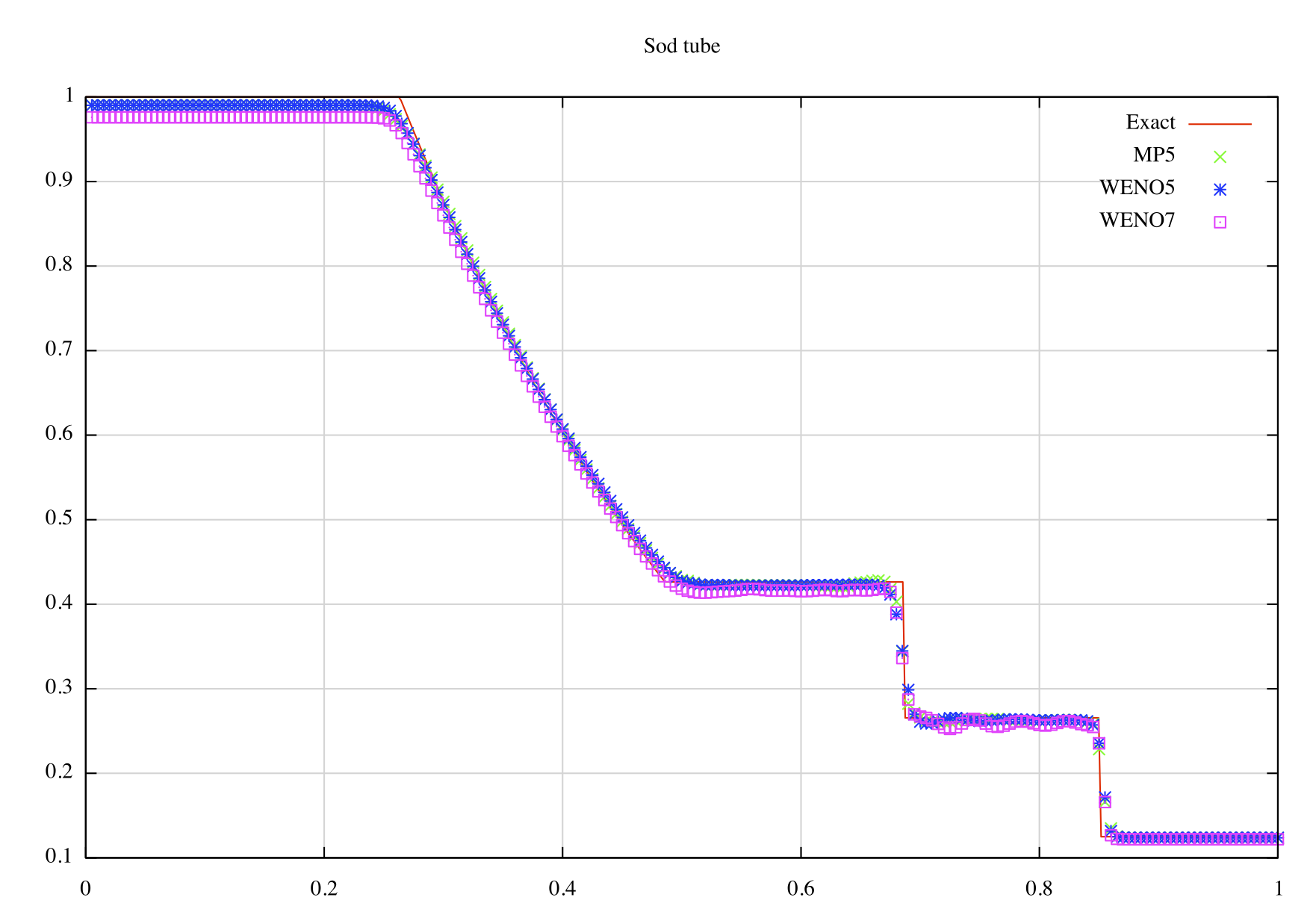This helps the situation a good deal and makes the time step selection or the wave speed estimate better, but far worse things can happen (the vacuum state issue mentioned above).

Here is the problem that causes this issue to persist. To really get your arms around this issue requires a very expensive solution to the Riemann problem, the exact Riemann solver. Moreover to get the bounding wave speed in general requires a nonlinear iteration using Newton’s method, and checking my own code 15 iterations of the solver. No one is going to do this to control time steps or estimate wave speeds.

Yuck!

I will postulate that this issue can be dealt with approximately. A first step would be to include the simplest nonlinear Riemann solver to estimate things; this uses the acoustic impedances to provide an estimate of the interior state of the Riemann fan. Here one puts the problem in a Lagrangian frame and solve the approximate wave curves, on the left side and on the right side solving for and . Then use the jump conditions for density, to find the interior densities (similar to the right). Then compute the interior sound speeds to get the bounds. The problem is that for a strong shock or rarefaction this approximation comes up very short, very short indeed.

The way to do better is to use a quadratic approximation for the wave speeds where the acoustic impedance changes to account for the strength of the interaction. I used these before to come up with a better approximate Riemann solver. The approximation is largely the same as before except, . Now you solve a quadratic problem, which is still closed form, but you have to deal with an unphysical root (which is straightforward using physical principles). For the strong rarefaction this still doesn’t work very well because the wave curve has a local minimum at a much lower velocity than the vacuum velocity.

I think this can be solved, but I need to work out the details and troubleshoot. Aside from this the details are similar to the description above.

Rider, William J. “An adaptive Riemann solver using a two-shock approximation.” Computers & fluids 28.6 (1999): 741-777.

An expert is someone who knows some of the worst mistakes that can be made in his subject, and how to avoid them.

One of my first talked about the Multimat2013, a biannual meeting of scientists specializing in the computation of multi-material compressible flows. Last time in 2013 we met in San Francisco, this time in Würzburg Germany. These conferences began as a minisymposium at an international congress in 2000. The first actual “Multimat” was 2002 in Paris. I gave the very first talk at this meeting (and it was a near disaster, an international jet lag tale with admonitions about falling asleep when you arrive in Europe, don’t do it!). The 2^nd Conference was in 2005 and then every two years thereafter. The spiritual leader for the meetings and general conference chairman is Misha Shashkov, a Lab fellow at Los Alamos. Still taken as a whole the meeting marks a remarkable evolution and renaissance for numerical methods, particularly Lagrangian frame shock capturing.

Sometimes going to a conference is completely justified by witnessing a single talk. This was one of those meetings. Most of the time we have to justify going to conferences by giving our own talks. The Multimat2015 conference was a stunning example of just how wrong-headed this point of view is. The point of going to a conference is to be exposed to new ideas from a different pool of ideas than you usually swim in. It is not to market or demonstrate our own ideas. This is not to say that giving talks at conferences aren’t valuable, they just aren’t the principle or most important reason for going. This is a key manner in which our management simply misunderstands science.

The morning of the second day I had the pleasure of seeing a talk by Michael Dumbser (University of Trento). I’ve followed his career for a while and deeply appreciate the inventive and interesting work he does. For example I find his PnPm methods to be a powerful and interesting approach to discretely attacking problems in a manner that may be vastly powerful. Nonetheless I was ill prepared for the magnificent work he presented at Multimat2015. One of the things that have held discontinuous Galerkin methods back for years is nonlinear stabilization. I believe Michael has “solved” this problem, at least conceptually.

Like many brilliant ideas he took a problem that cannot be solved well and recast it into a problem that we know how to solve. This is just such a case. The key idea is to identify elements that need nonlinear stabilization (or in other words, the action of a limiter). One identified, these elements are then converted into a number of finite volume elements corresponding to the degrees of freedom in the discontinuous basis used to discretize the larger element. Then a nonlinear stabilization is applied to the finite volumes (using monotonicity limiters, WENO, etc. whatever you like). Once the stabilized solution is found on the temporary finite volumes, the evolved original discontinuous basis is recovered from the finite volume solution. Wow what an amazingly brilliant idea! This provides a methodology that can retain high sub-element level resolution of discontinuous solutions.

The problem that remains are producing a nonlinear stabilization suitable for production use that goes beyond monotonicity preservation. This was the topic of my talk, how does one most to something better than mere monotonicity preservation as a nonlinear stabilization technique and be robust enough for production use. We need to produce methods that stabilize solutions physical, but retain accuracy to a larger degree while producing results robustly enough for use in a production setting. Once such a method is developed it would improve Dumbser’s method quite easily. A good step forward would be methods that do not damp isolated, well-resolved extrema in a robust way. Just as first order methods are the foundation for monotonicity preserving methods, I believe that monotonicity preserving methods can form the basis for extrema-preserving methods.

I often use a quote from Scott Adams to describe the principle for designing high-resolution methods, “Logically all things are created by a combination of simpler less capable components,” pointed out by Culbert Laney in his book Computational Gas Dynamics. The work of Dumbser is a perfect exemplar of this principle in many ways. Here the existing state of the art methods for Gas Dynamics are used as fundamental building blocks for stabilizing the discontinuous Galerkin methods.

Another theme from this meeting is the continued failure by the broader hyperbolic PDE community to quantify errors, or quantify the performance of the methods used. We fail to do this even when we have an exact solution… Well this isn’t entirely true. We quantify the errors when we have exact solution that is continuously differentiable. So when the solution is smooth we show the order of accuracy. Change the problem to something with a discontinuity and the quantification always goes away and replaced with hand-waving arguments and expert judgment.

The reason is that the rate of convergence for methods is intrinsically limited to first-order with a discontinuity. Everyone then assumes that the magnitude of the error is meaningless in this case. The truth is that the magnitude of the error can be significantly different from method to method and an array of important details changes the error character of the methods. We have completely failed to report on these results as a community. The archetype of this character is Sod’s shock tube, the “hello World” problem for shock physics. We have gotten into the habit of simply showing results to this problem that demonstrate that the method is reasonable, but never report the error magnitude. The reality is that this error magnitude can vary by a factor of 10 for commonly used methods at the same grid resolution. Even larger variations occur for more difficult problems.

The problems with a lack of quantification continue and magnify in more than one dimension. For problems with discontinuities there are virtually no exact solutions for problems in multiple dimensions (genuinely multi-dimensional as opposed to problems that are one-dimensional run in multiple dimensions). One of the key aspects of multiple dimensions is vorticity. This renders problems chaotic and non-unique. This only amplifies the hand waving and expert statements on methods and their relative virtues. I believe we should be looking for ways to move past this habit and quantify the differences.

This character in no small way is holding back progress. As long as hand waving and expert judgment is the guide for quality, progress and improvements for method will be hostage to personality instead of letting the scientific method guide choices.

General issues with quantifying the performance of methods. Where it is easy isn’t done, where it is hard. Multidimensional problems that are interesting all have vorticity, the results are all compared in the infamous eyeball or viewgraph norm. Mixing & vorticity are essential, but never measured. All comparisons are expert based and use hand-waving arguments, and the current experts and their methods will continue to hold sway and progress will wane.

The heart of excitement for previous meetings, collocated, cell-centered Lagrangian methods have now become so common and broadly used as to be passé. A number of good talks were given on this class of methods showing a broad base of progress. It is remarkable that such methods have now perhaps displaced the classical staggered mesh methods originating with Von Neumann as the stock and trade of this community. The constant and iterative progress with these methods awaits the next leap in performance, and the hard work of transitioning to being a workhorse in production solutions. This work is ongoing and may ultimately provide the impetus for the next great leap forward.

Aside from this work the meeting attempts to work within the natural tension between physics, mathematics, engineering and computer science to its great benefit. In addition to this beneficial tension, the meeting also straddles the practical and pragmatic needs of code developers for production software, and university research. Over the years we have witnessed a steady stream of ideas and problems flowing back and forth between these disparate communities. As such the meeting is a potpourri of variety and perspective providing many great ideas for moving the overall technical community forward through the creative utilization of these tensions

We tend to overvalue the things we can measure and undervalue the things we cannot.

Now I am looking forward to the next meeting two years hence in Santa Fe.

Some men are born mediocre, some men achieve mediocrity, and some men have mediocrity trust upon them.

― Joseph Heller

In taking a deep breathe and pausing from my daily grind, I considered the question, “what do we want from our Labs?” By Labs I mean the loose collection of largely government sponsored research institutions supporting everything from national defense to space exploration. By, we, I mean the Nation and its political, intellectual and collective leadership. Working at a Lab for the last 25 plus years under the auspices of the Department of Energy (working for two Labs actually), I think this question is worth a lot of deep thinking and consideration.

A reasonable conclusion drawn from the experiences given my span of employment would be,

“We want to destroy the Labs as competent entities.”

I’m fairly sure this isn’t the intent of our National Leadership, but rather an outcome of other desires. Otherwise well-intentioned directives that have deeply damaging unintended consequences drive the destruction of the Labs. While calling the directives well-intentioned is probably correct, the mindset driving them is largely a combination of fear, control and unremittingly short-term thinking. Such destruction is largely a consequence of changes in National behavior that sweep across every political and economic dimension. Many of the themes parallel the driving forces of inequality and a host of other societal transformations.

One of the key aspects of the Labs that deeply influenced my own decision to work there was their seemingly enduring commitment to excellence. In the years since, this commitment has wavered and withered to the point where excellence gets lip service and little else. The environment no longer supports the development or maintenance of truly excellent science and engineering (despite frequent protestations of being “World Class”). Our National Labs were once truly World Class, but no more. Decades of neglect and directives that conflict directly with achieving World Class results have destroyed any and all claim to such lofty status. We are not part of an acceptance of mediocrity that we willfully ignore and ignorantly claim to be excellent and world class.

World Class requires commitment to quality of the sort we cannot muster because it also requires a degree on independence and vigorous intellectual exchange that our masters can no longer tolerate. So, here is my first answer of what they want from the Labs,

“obedience” and “compliance”

above all else. Follow rules and work on what you are told to work on. Neither of these values can ever lead to anything “World Class”. I would submit that these values could only undermine and work to decay everything needed to be excellent.

One place where the fundamental nature of excellence and the governance of the Labs intersect is the expectations on work done. If one principle dominates the expectations that the Labs must comply with is

“do not ever ever ever fail at anything”.

The kneejerk response from politicians, the public and the increasingly scandal-mongering media is “that seems like a really good thing.” If they don’t fail then money won’t be wasted and they’ll just do good work. Wrong and wrong! If we don’t allow failure, we won’t allow success either, the two are intertwined as surely as life and death.

In reality this attitude have been slowly strangling the quality from the Labs. By never allowing failure we see a march steadily toward mediocrity and away from excellence. No risks are ever taken, and the environment to develop World Class people, research and results is smothered. We see an ever-growing avalanche of accounting and accountability to make sure no money ever gets wasted doing anything that wasn’t pre-approved. Meticulous project planning swallows up any and all professional judgment, risk-taking or opportunities. Breakthroughs are scheduled years in advance, absurd as that sounds.

People forget how fast you did a job – but they remember how well you did it

― Howard Newton

The real and dominant outcome from all this surety of outcomes is a loss of excellence, innovation and an ever-diminishing quality. The real losers will be the Nation, its security and its economic vitality into the future. Any vibrancy and supremacy we have in economics and security is the product of our science and technology excellence thirty to forty years ago. We are vulnerable to be preyed upon by whomever has the audacity to take risks and pursue the quality we have destroyed.

Another piece of the puzzle are the salaries and benefits for the employees and managers. At one level it is clear that we are paid well, or at least better than the average American. The problem is that in relative terms we are losing ground every year to where we once were. On the one hand we are told that we are World Class, yet we are compensated at a market-driven, market-average rate. Therefore we are either incredibly high-minded or the stupidest World Class performers out there. At the same time the management’s compensation has shot up, especially at the top of the management of the Labs. On the one hand this is simply an extension of the market-driven approach. Our executives are compensated extremely well, but not in comparison to their private industry peers. In sum the overall picture painted by the compensation at the Labs is one of confusion, and priorities that are radically out of step with the rhetoric.

All of this is tragic enough in and of itself were it simply happening at the Labs alone. Instead these trends merely echo a larger chorus of destruction society wide. We see all our institutions of excellence under a similar assault. Education is being savaged by many of the same forces. Colleges view the education of the next generation as a mere afterthought to balancing their books and filling their coffers. Students are a source of money rather than a mission. One need only look at what universities value; one thing is clear educating students isn’t their priority. Business exists solely to enrich their executives and stockholders; customers and community be damned. Our national infrastructure is crumbling without anyone rising to even fix what already exists. Producing an infrastructure suitable for the current Century is a bridge too far. All the while the Country pours endless resources into the Military-Industrial Complex for the purpose of fighting paper tigers and imaginary enemies. Meanwhile the internal enemies of our future are eating us from within and winning without the hint of struggle.

In the final analysis what are we losing by treating our Labs with such callousness and disregard? For the most part we are losing opportunity to innovate, invent and discover the science and technology of the future. In the 25 years following World War II the Labs were an instrumental set of institutions that created the future and continued the discoveries that drove science and technology. The achievements of that era are the foundation of the supremacy in both National defense and security, but also economic power. By destroying the Labs as we are doing, we assure that this supremacy will fade into history and we will be overtaken by other powers. It is suicide by a slow acting poison.

Quality means doing it right when no one is looking.

― Henry Ford

We have short-circuited the engines of excellence in trying to control risk and demonstrate accountability. The best way to control risk is not take any. We have excelled at this. By not taking risks we don’t have to deal with or explain failure in the short-term, but in the long-term we destroy quality and undermine excellence. Accountability is the same. We know how every dollar is spent, and what work is done every hour of the day, but that money no longer supports serendipity and the professional discretion and judgment that underpinned the monumental achievements of the past. One cannot claim to plan or determine a priori the breakthroughs and discoveries they haven’t made yet. Now we simply have low-risk and fully accountable Laboratories that can only be described as being mediocre.

Such mediocrity provides the Nation with no short-term issues to explain or manage, but makes our long-term prospects clearly oriented towards a decline in the Nation’s fortunes. We seem to uniformly lack the courage and ethical regard for our children to stop this headlong march away from excellence. Instead we embrace mediocrity because it’s an easy and comfortable short-term choice.

We don’t get a chance to do that many things, and every one should be really excellent. Because this is our life.

― Steve Jobs

The only sin is mediocrity.

― Martha Graham

We’ve taken the world apart but we have no idea what to do with the pieces.

― Chuck Palahniuk

There are a lot of ways to turn differential equations into a discrete system and numerical solve them. The choices usually come down to three different, but slightly ambiguous choices, finite differences, finite volumes, or finite elements. One of the important, but fuzzy pieces of knowledge is the actual meaning of the variables you’re solving in the first place. Some clarity regarding the variables detailed identity can come in handy, if not be essential to high fidelity solution. With any luck we can shed some light on this.

The place to start is writing down the governing (usually differential) equations. If your problem is geometrically complex, finite element methods have a distinct appeal. The finite element method has a certain “turn the crank” approach that takes away much of the explicit decision-making in discretization, but the decision and choices are so much deeper than this if you really care about the answer.

Tiny details imperceptible to us decide everything!

― W.G. Sebald

I’ve never been a fan of not thinking deeply about what you are doing at a very specific way. Finite element aficionados seem to be very keen on avoiding as much thought as possible in discretization with a philosophy of choosing your element and associated shape functions and letting the chips fall where they may. For simple problems with a lot of regularity (smoothness) this can work well and even be advantageous, but for difficult problems (i.e., hyperbolic PDEs) this can be disastrous. In the end people would be far better served by putting more thought into the transition from the continuous to the discrete.

My recent posts have been examples of the sorts of details that really matter a lot in determining the quality of results in computing. Ideas like convergence, limiting solutions, dissipation, and accuracy all matter a tremendous degree and make the difference between stability and instability, high and low fidelity, run of the mill and state of the art, and ultimately high quality. Failure to pay acute attention to the details of the discretization will result in mediocrity.

It should come as no surprise that I don’t particularly care for the finite element method, so in keeping with my tastes I’m focusing on the finite volume and finite difference methods today. There are significant differences between the two that should be taken into account when deriving discrete approximations. Perhaps more interestingly, there is a fairly well defined way to translate between the two points of view. This translation makes for a useful addition to anyone’s discretization “toolbox”.

Once upon a time there was no such thing as the “finite volume method” it was simply a special finite difference method. Some finite differences employed a discrete conservation principle, and could be thought of as directly updating conserved quantities. These distinctions are not terribly important until methods become higher than second-order in order of accuracy. Gradually the methodology became distinct enough that it was worth making the distinction. The term “finite volume” came into the vernacular in about 1973 and stuck (an earlier paper in 1971 coined “finite area” method in 2-D).

The start of the distinctions between the two approaches involves how the equations are updated. For a finite difference method the equations should be updated using the differential equation form of the equations at a point in space. For a finite volume method the equations should be updated in a manner consistent with an integral conservation principle for a well-defined region. So the variables in a finite difference method are defined at a point, and the values in a finite volume method are defined as the integral of that quantity over a region. Transfers between adjoining regions via fluxes are conserved, what leaves one volume should enter the next one. Nothing about the finite difference method precludes conservation, but nothing dictates it either. For a finite volume method conservation is far more intrinsic to its basic formulation.

Consider a conservation law, . One might be interested in approximating with either finite differences or finite volumes. Once a decision is made, the approximation approach falls out naturally. In the finite difference approach, one takes the solution at points in space (or in the case of this PDE, the fluxes, ) and interpolates these values in some sort of reasonable manner. Then the derivative of the flux is evaluated. The update equation is then . This then can be used to update the solution by treating the time like an ODE integration. This is often called the “method of lines”.

For a finite volume method the approach is demonstrably different. The update of the variable makes explicit contact with the notion that it is a quantity that is conserved in space. For the simple PDE like that above the update equation requires the updating of the variables with fluxes computed at the edge of the cell. Notice that the fluxes have to be evaluated at the edges, which can assure that the variable, is conserved discretely. The trick to doing the finite volume method properly is the conversion of the set of cell (element) conserved values of to the point values at the edges as fluxes. It isn’t entirely simple. Again an interpolation can be utilized to achieve this end, but the interpolation form must adhere to the character of the conservation of the variable. Thus when the interpolant is integrated over the cell it must return the conserved quantity in that cell precisely. This can be accomplished through the application of the classical Legendre polynomial basis for example.

Perhaps you’re now asking about how to translate between these two points of view. It turns out to be a piece of cake. It is another useful technique to place into the proverbial toolbox. It turns out that the translation between the two can be derived from the interpolations discussed about and rightfully mirrors each other. If one takes a set of control volume, integrally averaged, values and recovers the corresponding point values the formula is remarkably simple. Here I will refer to control volume values by and the point values by . Then we can transform to point values via . The inverse operation is and is derived by integrating the point wise interpolation over a cell. For higher order approximations these calculation are a bit more delicate than these formula imply!

For finite element methods we usually have the standard flavor of the continuous finite elements. Thinking about the variables in that case they are defined by nodal values, the “shape function” describing their variation in space, and its appropriately weighted integral. A more modern and exciting approach is discontinuous Galerkin, which does not require continuity of solution across element boundaries. The lowest order version of this method is equivalent to a low-order finite volume scheme. The variable is the zeroth moment of the solution over a cell. One way of looking at high order discontinuous Galerkin methods is taking successive moments of the solution over the cells (elements). This method holds great promise because of its high fidelity and great locality.

This is just the start of this exploration, but the key is know what your variables really mean.

Little details have special talents in creating big problems!

― Mehmet Murat ildan

Here, I will provide some concepts that may spur further development through attacking each of these three shortcomings in newer methods. Part of the route to analysis is utilization of evolution equations and the analysis of numerical methods using modified equation analysis. These concepts were essential in ideas that were key in the formulation of the original generation of (linear) monotone methods [HHL76] and revisiting these concepts should provide impetus for new advances. The approach is two-fold: explain why current methods are favored and provide a catalog of characteristics for new methods to follow.

In the past, I have used modified equation analysis in the past to unveil the form of the subgrid modeling provided by high-resolution methods for large eddy simulation (the so-called MILES or Implicit LES approach). This approach has provided a systematic approach to providing explanations for the effectiveness of high-resolution methods for modeling turbulence by revealing the implied subgrid model in implicit in the methods.

In solving hyperbolic conservation laws the work of Lax [Lax73] is preeminent. Lax identified the centrality of conservation form to computing weak solutions (along with Wendroff) [LW60]. Once weak solutions are achieved, it is essential to produce physically admissible solutions, which the concept of vanishing viscosity provides. Harten, Hyman and Lax [HHL76] provided the critical connection to numerical methods by showing that upwind differencing provided physically admissible solutions utilizing the method of modified equations to the analysis of the numerical method (the same can be shown for Lax-Friedrichs-based methods). These methods form the foundation upon which high-resolution methods are based.

Of course while these theoretical developments were made parallel discoveries were happening in the first high-resolution methods. Independently three different researchers discovered the basic principle of high-resolution methods, nonlinear selection of computational stencils so that the method becomes nonlinear even for linear problems [Boris71,VanLeer72,Kolgan72]. Each method allowed the barrier theorem of Godunov [God59] to be overcome and paved the way for further developments. Ultimately, Harten provided the work to tie these streams of work together by introducing the total variation concepts to formalize the mathematics [Harten83]. These methods form a foundation for a renaissance in numerical hyperbolic conservation laws.

Subsequently, there have been several attempts to move beyond the first generation of high resolution methods, but each has met with limited success [HEOC87,Shu87]. While this work has yielded some practical methods, none has shared the extreme success of the initial set of methods and their basis in mathematics. These methods have not yielded the same quantum leap in performance as the original methods, and not met the same success in being ubiquitous in applications. The reasons for this practical failure are multiple chiefly being cost, fragility, and failure of formal high-order accuracy to yield practical accuracy. I studied some of these basic tradeoffs with Jeff Greenough [GR04] between archetypical methods PLM [CG85] and fifth-order WENO [JS95].

The trick to forgetting the big picture is to look at everything close up.

I am proposing revisiting the foundational aspects of high-resolution methods by returning to modified equation analysis of numerical methods and providing connections to providing proof of physically admissible solutions, and their control of variation in the solution (i.e., connecting to variation-diminishing properties). To conduct such analysis I am suggesting the study of the energy evolution of equations, and/or the continuous variation evolution. Each equation will admit a vanishing viscosity solution, and the modified equation analysis can provide a connection of the numerical method to admissibility. The properties of the vanishing viscosity solution define the nature of desirable results. For a simple hyperbolic PDE, , the basic physical admissibility condition can be given . 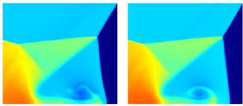For higher order methods, the viscosity must be nonlinear and a function of the solution itself. Similarly the variation evolution may be derived and its vanishing viscosity solution can be similarly stated. In the rest of the discussion here, we will focus on the linear version of the equation for simplicity, .

When modified equation analysis is applied to upwind differencing, the classical result can be easily derived for the numerical viscosity, . For the variation equation the result is similar, but informative, . We can see that the term proportional to is positive negative and will reduce the variation where ever the sign of variation changes.

If we analyze classical TVD method using the minmod limiter, the connection to physical admissibility becomes clear for the kinetic energy evolution, . Similarly the variation evolution provides a similar connection with more texture on the nature of the solution with the leading truncation error term being a flux . When expanding the flux in the modified differential equation, two terms emerge as being non-conservative of variation, . The second term is negative definite while the first term could be either positive or negative. We would categorize the scheme as being quite likely to be variation diminishing, but not absolutely. Discretely, we know that the method is TVD. Note that the viscosity coefficient, , is now a nonlinear function of the solution itself and could be called a “hyper-viscosity”. It is important that the actual discrete scheme limits the magnitude of this ratio to one, so the ratio does not blow up in practice.

We can apply the same technique to ENO or WENO methods and see the nature of its regularization at least for smooth solutions. For the famous fifth-order WENO we can derive the modified equation for the kinetic energy and find the leading order viscosity coefficient , a nonlinear and linear hyper-viscous regularization. For the variation evolution the variation changing terms are . The middle term is negative definite, but the first and third terms will be ambiguous for variation diminishment. This sort of behavior is observed for this scheme with the variation both shrinking and growing as time advances. Perhaps more importantly, the fully discrete method does not limit the size of the hyper-viscosity and it could blow up. The nonlinear hyperviscosity is itself ambiguous in terms of its variation diminishing character, which is distinctly different than the TVD scheme.

For the classical ENO scheme the result is quite similar. In the classical ENO scheme, the smoothest stencil is chosen hierarchically starting with first-order upwind. In other words the second order scheme is chosen to be the closest to the first-order scheme and the third-order stencil is chosen that is closest to the second-order stencil. We can analyze the third-order version using modified equation analysis. The effective numerical viscosity is a combination on linear and nonlinear hyperviscosity, . This can be analyzed for the variation equation and produces ambiguously signed non-conservative terms, . We find that ENO is quite similar to WENO, and the hyperviscosity magnitude is not controlled by the nonlinearity in the method. Practically speaking this is a deep concern when considering the robustness of the method.

The last method we analyze is one that I have suggested as a path forward. In a nutshell it is the high order method that is closest to a certain TVD method in some sense (I use the value of edge fluxes). Importantly, this method can still degenerate to the first-order upwind scheme while being formally third-order accurate. If the TVD method is chosen to be the first-order upwind method, we can analyze the result. The nonlinear dissipative flux is a third-order method, . For the variation equation we get a remarkably simple non-conservative term that is negative definite, . This is an extremely hopeful form indicating excellent variation properties while retaining high order.

The modified equation analysis is enabled by a combination of symbolic algebra (Mathematica) and certain transformations formerly utilized to analyze implicit large eddy simulation [MR02,RM05,GMR07].

Finally, we can utilize these methods to produce a new class of methods that offer the promise of greater resolution and more provable connections to physical admissibility. The basic concept is to use TVD methods (and their close relatives) to ground high-order discretizations. The higher order approximations will be chosen to be closest to the TVD method is a well-defined sense. Through these means we can assure that the high-order method simultaneously provides accuracy and variation control by analyzing the resulting schemes via modified equation analysis. These methods will typically have similar regularizations to the WENO methods and provide high resolution results that are both formally accurate when appropriate and higher resolution than the TVD methods they are grounded by. For a third-order method the analysis of this method provides the following results for the kinetic energy equation, and the variation evolution. I believe this approach will provide a beneficial path for method development and analysis.

Out of clutter, find simplicity.

If you’re not confused, you’re not paying attention.

[Harten83] Harten, Ami. “High resolution schemes for hyperbolic conservation laws.”Journal of computational physics 49, no. 3 (1983): 357-393.

[HEOC87] Harten, Ami, Bjorn Engquist, Stanley Osher, and Sukumar R. Chakravarthy. “Uniformly high order accurate essentially non-oscillatory schemes, III.” Journal of computational physics 71, no. 2 (1987): 231-303.

[HHL76] Harten, Amiram, James M. Hyman, Peter D. Lax, and Barbara Keyfitz. “On finite‐difference approximations and entropy conditions for shocks.”Communications on pure and applied mathematics 29, no. 3 (1976): 297-322.
[LW60] Lax, Peter, and Burton Wendroff. “Systems of conservation laws.”Communications on Pure and Applied mathematics 13, no. 2 (1960): 217-237.

[Lax73] Lax, Peter D. Hyperbolic systems of conservation laws and the mathematical theory of shock waves. Vol. 11. SIAM, 1973.

[Boris71] Boris, Jay P., and David L. Book. “Flux-corrected transport. I. SHASTA, A fluid transport algorithm that works.” Journal of computational physics 11, no. 1 (1973): 38-69.

(Boris, Jay P. A Fluid Transport Algorithm that Works. No. NRL-MR-2357. NAVAL RESEARCH LAB WASHINGTON DC, 1971.)

[VanLeer73] van Leer, Bram. “Towards the ultimate conservative difference scheme I. The quest of monotonicity.” In Proceedings of the Third International Conference on Numerical Methods in Fluid Mechanics, pp. 163-168. Springer Berlin Heidelberg, 1973.

[Kolgan72] Kolgan, V. P. “Application of the minimum-derivative principle in the construction of finite-difference schemes for numerical analysis of discontinuous solutions in gas dynamics.” Uchenye Zapiski TsaGI [Sci. Notes Central Inst. Aerodyn] 3, no. 6 (1972): 68-77.

(van Leer, Bram. “A historical oversight: Vladimir P. Kolgan and his high-resolution scheme.” Journal of Computational Physics 230, no. 7 (2011): 2378-2383.)

[God59] Godunov, Sergei Konstantinovich. “A difference method for numerical calculation of discontinuous solutions of the equations of hydrodynamics.”Matematicheskii Sbornik 89, no. 3 (1959): 271-306.

[Shu87] Shu, Chi-Wang. “TVB uniformly high-order schemes for conservation laws.”Mathematics of Computation 49, no. 179 (1987): 105-121.

[GR04] Greenough, J. A., and W. J. Rider. “A quantitative comparison of numerical methods for the compressible Euler equations: fifth-order WENO and piecewise-linear Godunov.” Journal of Computational Physics 196.1 (2004): 259-281.

[CG85] Colella, Phillip, and Harland M. Glaz. “Efficient solution algorithms for the Riemann problem for real gases.” Journal of Computational Physics 59.2 (1985): 264-289. & Colella, Phillip. “A direct Eulerian MUSCL scheme for gas dynamics.” SIAM Journal on Scientific and Statistical Computing 6.1 (1985): 104-117.

[JS95] Jiang, Guang-Shan, and Chi-Wang Shu. “Efficient Implementation of Weighted ENO Schemes.” Journal of Computational Physics 1.126 (1996): 202-228.

[GLR07] Grinstein, Fernando F., Len G. Margolin, and William J. Rider, eds. Implicit large eddy simulation: computing turbulent fluid dynamics. Cambridge university press, 2007.

[RM05] Margolin, L. G., and W. J. Rider. “The design and construction of implicit LES models.” International journal for numerical methods in fluids 47, no. 10‐11 (2005): 1173-1179.

[MR02] Margolin, Len G., and William J. Rider. “A rationale for implicit turbulence modelling.” International Journal for Numerical Methods in Fluids 39, no. 9 (2002): 821-841.

Linearity Breeds Contempt

— Peter Lax

The development of high-resolution numerical methods for hyperbolic conservation laws has been an outstanding achievement for computational physics. These methods have provided an essential balance of accuracy (fidelity or resolution) with physical admissibility with computational tractability. While these methods were a tremendous achievement, their progress has stalled in several respects. After a flurry of development, the pace has slowed and adoption of new methods into “production” codes has come to a halt. There are good reasons for this worth exploring if we wish to see if progress can be restarted. This post builds upon the two posts from last week, which describes tools that may be used to develop methods.

Things have stalled for the very reasons that the adoption was so rapid and complete. The sort of radical success that the high-resolution (monotonicity-preserving) methods experienced may be difficult to impossible to replicate with new methods. The biggest thing that the monotonicity-preserving methods did was change the fundamental nature of the numerical viscosity from a form that inherently computed laminar, syrupy-looking flows to a numerical viscosity that allowed flows to take on an energetic character that gives fluid dynamics is power and beauty.

Why did the resolution simply stop at the rise from first- to second-order methods? One reason is probably deeply connected to the fundamental nature of nonlinear fluid systems and their inherent dissipation when viscosity is small. As it turns out the canonical small viscosity structures in flows, shocks and turbulence exhibit the same general form for the scaling of dissipation in these cases. Both show a dissipation that is proportional to the change in velocity in the direction of the flow cubed (the normal or longitudinal velocity). The fundamental numerical error for a second-order method in conservation (or control volume) form produces the correct asymptotic nonlinear dissipation of flow energy into heat. The monotonicity-preserving numerical methods allowed this term to achieve prominence in solutions helping to produce more physical appealing solutions.

The issue is that newer methods need to cure smaller ills in the current solutions. Sometimes monotonicity is not the right thing to enforce, and extreme values in the solution are damped severely, and shapes are greatly distorted. These problems are important, but not nearly as profound as the set of issues that monotonicity-preserving methods cured. We cannot expect the same level of transformative solution improvement. The case for adopting any newer methods is bound to be more subtle and less clear cut. Existing approaches that improve on monotonicity preservation are generally quite expensive without providing a commensurate improvement in solution quality.

Moreover the improvements in the solution from the new methods are generally highly subjective and lack a quantitative edge. At best, the case for using them is highly subjective and far from clear-cut. Adding to the problems are two key aspects in numerical analysis that further cloud and undermine the case for advancing. First, solutions are inherently lacking sufficient smoothness to give high-order accurate methods the full benefit of their properties. Secondly, the stability of the newer methods is substantially less than the adopted generation of methods, which provide almost as much robustness as the first-order methods they easily displaced. The newer methods are far too fragile for production codes. Part of the reason for this is the tendency to eschew every using the first-order approximation even locally. Thirdly the nonlinear stability principle associated with the newer methods is far weaker than monotonicity preservation and sometimes even precipitates new modes of instability in the solution.

Three strikes and you’re out

— A rule in Baseball, the “American Pastime”

Now we can revisit the three main issues for the new methods and provide suggestions that may allow progress to begin anew. The three shortcomings I identified above are the following:

1. Lack of smoothness, and full utility for high-order accuracy
2. Removal of the first-order method as a robustness mechanism
3. A much weaker nonlinear stability principle, and new potential instabilities

It might be useful to revisit some old advise from Bell, Colella and Trangenstein [BCT89] before unveiling my suggestions on principles to use in developing high resolution methods using monotoncity preservation,

1. Use a good foundational high-order method, upstream centered, or high-order centered
2. Use an entropy satisfying Riemann solver
3. Add additional dissipation at strongly nonlinear or degenerate discontinutities.

These maxims are closely related to the reasons why this class of methods has been so successful:

1. Solutions are monotonicity preserving without inducing linear laminar viscosity and replacing it with a hyper viscosity that provides more energetic physically meaningful solutions,
2. It unveils the prominence of the control volume term, which provides an asymptotically appropriate stabilizing nonlinear dissipation term,
3. When the solution is significantly under-resolved or in-danger of unphysical solutions use a first-order methods as a “safety net”.

Putting all of these considerations into account and then thinking about how to move past the current state-of-the-art. We need to account for the weaknesses of current methods and advance beyond monotonicity preservation into account, and other advice, I can write down my three suggestions (keeping BCT’s advise as a base):

1. Base the nonlinear stability principle on monotonicity-preservation with detection of extrema and careful relaxation of those conditions
2. Continue to use the high-order base method unless it produces a distinct monotonicity violating solution.
3. Careful analysis of strongly nonlinear discontinuities to assure that the approximation is locally nonlinearly stable. If the solution is highly under-resolved give up high-order accuracy and degenerate to first order.

Next week I’ll unveil some new analysis that sheds light on how the methods work based on modified equation analysis. It also points to some details of what might work in the future.

[BCT89] Bell, John B., Phillip Colella, and John A. Trangenstein. “Higher order Godunov methods for general systems of hyperbolic conservation laws.” Journal of Computational Physics 82.2 (1989): 362-397.

[Hersh] Hersh, Reuben. Peter Lax, Mathematician: An Illustrated Memoir. Vol. 88. American Mathematical Soc., 2014.

[Lax1978] Lax, Peter D. “Accuracy and resolution in the computation of solutions of linear and nonlinear equations.” Selected Papers Volume I (2005): 184-194.

Boundary violations are deeply experienced.

― David W. Earle

The post yesterday is closely connected to this one.

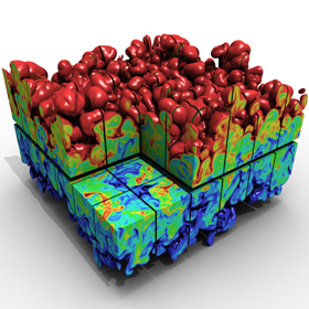
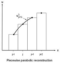
Yesterday I talked about a general purpose form for “limiters” applied to polynomial reconstructions, . For methods of this type the reconstruction is important because it defines the value of the function where there is not data, at cell-edges or faces where fluxes are computed, . For a method in conservation form the edge-face values are essential to updating the solution. As I will discuss the value of these values and mindful modifications of the values are severely under-utilized in implementing methods. Various methods can be improved in terms of accuracy, resolution, dissipation and stability through the techniques discussed in this post.

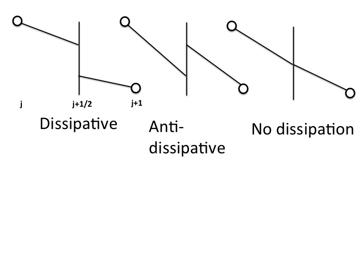
All of these techniques will utilize an important observation for methods of this type; one can swap edge-face values without impacting the accuracy of the method. Consider the reconstructed edge value that can (usually) be two values with a reconstruction being applied to $p\left(\theta_j \right)$ and $ p\left(\theta_{j+1} \right)$. If both reconstructions have equal accuracy we could trade these values, or replace one value by the other without impacting accuracy. Other properties like stability, dissipation or phase error are effected by this change, but formal accuracy is preserved.

One of the key aspects of the use of these edge values is a model for what an upwind method looks like applied to the data. Consider a nonlinear flux where upwinding will be applied to the edge values from two neighboring cells to determine the physically admissible flux, . An upwind approximation will use edge values from cells and . The simplest and most useful approximation of the flux is where is an eigen-decomposition of the flux Jacobian. The numerical dissipation is proportional to the eigenvalues and the jump at the cell edge . Generally speaking the physical direction of dissipation is defined by the jump from the cell-center (average) values, $latex– u_j $. The extrapolated edge values can (often) change the sign of the jump meaning that the approximation is locally anti-diffusive. A picture of faces is worth showing so one can understand what each swap looks like and envision the impact.

Perhaps the first application of this idea was the contact steepener defined by Colella and Woodward in their PPM method. Material interfaces also known as contact discontinuities are infamously diffused by Eulerian finite volume schemes even ones as high-resolution as PPM. The method introduced with PPM removes most of the diffusion usually induced by the method. The method works by locating valid interfaces and in the cells with the interface swapping the interface values at the edges. Often a material interface will be dissipative and swapping the edge values will be anti-diffusive. It is essential to apply a nonlinear stability mechanism to the swapped interface values and the polynomial reconstruction so that the anti-dissipative effects are not destabilizing. A second word of caution is the ill-advised nature of applying this technique at a nonlinear discontinuity such as a shock or rarefaction. For those flow features this technique would invite disaster.

A second, far safer application of edge swapping would be increasing the dissipation. In cases where the high-order local dissipation is anti-dissipative because the extrapolated values at the edges have a differently signed jump across the interface, swapping the edge values would make this dissipative. This condition has recently been dubbed as “entropy stable”. The condition can be computed by checking whether the jump in edge values has the same sign as the jump in cell-centered values . This should be particularly important in stably and physically moving nonlinear structures on the grid.  A concern is that too much dissipation is created as the figure shows. In this case the jump is entropy stable, but larger than the first-order method. This could actually be unstable especially if a Lax-Friedrichs flux is used because it is more dissipative than upwinding.

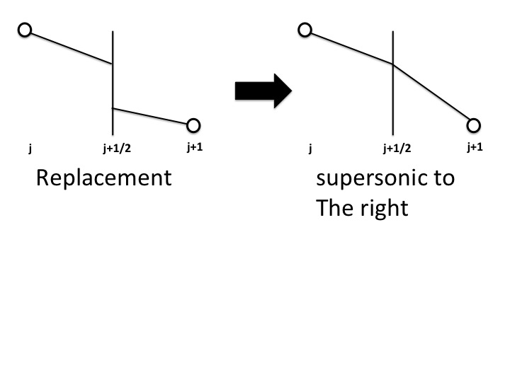
The penultimate approach would be to use these techniques to remove dissipation entirely from the edge. This is enabled by simply setting the two edge values to be equal in value. Any convex average of the edge values would achieve this as well as simply over-writing one of the edge values by the other. Like the anti-dissipative methods this would need to be applied with care for the stability of the overall integration procedure. In several cases the resulting approximation is actually higher order accurate. For example by applying this to first-order upwinding, the approximation is promoted to second-order central differencing. This happens for odd-ordered upstream centered methods, i.e., the third-order upwind methods is promoted to fourth-order centered edge values, the fifth-order upwind to sixth-order centered, and so forth.

The final approach to discuss would simply take one of the edge values and completely replace it by the other. The most obvious way to achieve this would be to declare that the information at the edge is unambigiously one-directional, and use that direction to choose the edge values. In this case one would short-circuit the Riemann solver and would only be stable for super-sonic flow. Of course, the opposite would produce a demonstrably anti-diffusive effect and might be useful (and dangerous too).

Don’t live a normal life by default, push the boundaries of your potential.

― Steven Redhead

Colella, Phillip, and Paul R. Woodward. “The piecewise parabolic method (PPM) for gas-dynamical simulations.” Journal of computational physics 54.1 (1984): 174-201.

Yang, Huanan. “An artificial compression method for ENO schemes: the slope modification method.” Journal of Computational Physics 89.1 (1990): 125-160.

Balsara, Dinshaw S., and Chi-Wang Shu. “Monotonicity preserving weighted essentially non-oscillatory schemes with increasingly high order of accuracy.”Journal of Computational Physics 160.2 (2000): 405-452.

Fjordholm, Ulrik S., Siddhartha Mishra, and Eitan Tadmor. “Arbitrarily high-order accurate entropy stable essentially nonoscillatory schemes for systems of conservation laws.” SIAM Journal on Numerical Analysis 50.2 (2012): 544-573.

Banks, Jeffrey William, and Jeffrey Alan Furst Hittinger. “A new class of nonlinear finite-volume methods for Vlasov simulation.” Plasma Science, IEEE Transactions on 38.9 (2010): 2198-2207.

Dumbser, Michael, and Olindo Zanotti. “Very high order P N P M schemes on unstructured meshes for the resistive relativistic MHD equations.” Journal of Computational Physics 228.18 (2009): 6991-7006.

Munz, Claus-Dieter, et al. “Enhanced Accuracy for Finite-Volume and Discontinuous Galerkin Schemes via Non-intrusive Corrections.” Recent Developments in the Numerics of Nonlinear Hyperbolic Conservation Laws. Springer Berlin Heidelberg, 2013. 267-282.

You can only exceed your limits if you’ve discovered them.

― Roel van Sleeuwen

About 15 years ago I wrote a simple paper with Len Margolin about options for modifying limiters used in high resolution schemes. Generally the paper didn’t get the success it deserved like so much else. It was studied by folks at Brown University, and was repurposed as a general positivity limiter. I will grant that the researchers at Brown did some really good work with the limiter especially proving how it could preserve accuracy (the positivity preserving limiter also preserves the design accuracy of the original reconstruction). I returned to this form in one of my recent papers, “Reconsidering Remap Methods” published earlier this year and the topic of a number of blog posts. Last week I realized that even more can be done with it and the form is really convenient for expressing a wide variety of nonlinear stability mechanisms in a more uniform manner.

The moment that crystalized my thinking was a re-reading and analysis of a limiter devised my Phil Colella and Michael Sekora for the PPM algorithm. This limiter was a “competitor” to an entirely different “limiting” strategy that I worked with Jeff Greenough and Jim Kamm. I now realized that the two limiters could be written in very nearly identical ways. Moreover, both of these ideas can be viewed as rather direct decedents of work by HT Huynh and Suresh from the late 1990’s. Each method attempts to extend nonlinear stability ideas beyond simply preserving monotonicity, to preserving valid extrema in solutions. Monontonicity preservation has the problem of seriously damping extrema with the limiter. All of these limiters can be expressed as different choices for a common form allowing direct comparison or mix and match ideas to be utilized effectively.

So, what is this common form?

Given a polynomial (or more general functions perhaps) representation of a solution in a computational cell, where , the limiter is implemented as , is the general limiter and . The limiter has a general form, . The “Standard” is the test that defines the nonlinear control of the solution while “Reconstruction Choice” is the feature being controlled. I will give some examples below. It is important to note that is the reconstruction that produces an upwind scheme that is the canonical linear monotonicity preserving (positive) method, but only first-order accurate. Higher order polynomials can be defined for higher accuracy, but without the limiter they are invariably oscillatory.

The most common choice is the definition of a positivity preserving limiter. In this case where is the lowest value of that will be tolerated for physical reasons. Next our reconstruction is interrogated .

The same can be done for monotonicity-preserving limiters. Here the most common application is “slope-limiting” where a common choice is here is the famous minimum modulus function that returns the smallest magnitude argument if the arguments have the same sign. where is the “high-order” slope that you desire to use and control the stability of.

For extrema preservation I will provide a couple of choices from my own work and Colella & Sekora. In both cases the extrema preservation will only be applied if a local extrema is detected by the scheme. Generally speaking a monotonicity preserving limiter will help do this by setting .

The idea that I worked on had a couple of key concepts: don’t give up on the original high-order scheme yet, at an extrema a ENO or WENO scheme might be useful, and the monotonicity preserving method has good nonlinear stability properties. My limiter worked on edge values that then helped define the reconstruction polynomial. It turns out that the general limiter can work here too, , and everything else follows. The parts of the limiter are with being the monotonicity preserving edge value, is the high-order edge values and is the WENO edge value. Next, the limiter is completed with . Part of the key idea is to use two complimentary nonlinear stability properties from monotonicity preservation and WENO to assure the stability of the method should the high-order method be chosen. In this case the high-order method is bounded by two nonlinearly stable approximation choices. I thought it actually worked pretty well.

Colella and Sekora had a different approach based on looking at the local curvature (second derivative) of the parabolic reconstruction used in PPM. If the second derivatives of the reconstruction and the neighborhood of the reconstruction all have the same sign and roughly the same magnitude, the extrema is viewed as valid and worth propagating undistorted by the sort of damping monotonicity preserving methods produce. A simple way to implement this approach can be implemented using the general limiter I discuss. First we need to define the second derivative of the polynomial reconstruction . In this case the specifics of the limiter are where is the classical second derivative on the mesh and . The choice of method to define the denominator in the limiter is . The resulting limiter can either be applied to the edge values or equivalently to the reconstructing polynomial.

In my next post I will talk about how edge values, can be used productively to improve the robustness, resolution and stability of these methods.

Set Goals, not Limits.

― Manoj Vaz

Rider, William J., and Len G. Margolin. “Simple modifications of monotonicity-preserving limiter.” Journal of Computational Physics 174.1 (2001): 473-488.

Qiu, Jianxian, and Chi-Wang Shu. “A Comparison of Troubled-Cell Indicators for Runge–Kutta Discontinuous Galerkin Methods Using Weighted Essentially Nonoscillatory Limiters.” SIAM Journal on Scientific Computing 27.3 (2005): 995-1013.

Zhang, Xiangxiong, and Chi-Wang Shu. “Maximum-principle-satisfying and positivity-preserving high-order schemes for conservation laws: survey and new developments.” Proceedings of the Royal Society of London A: Mathematical, Physical and Engineering Sciences. The Royal Society, 2011.

Zhang, Xiangxiong, and Chi-Wang Shu. “On maximum-principle-satisfying high order schemes for scalar conservation laws.” Journal of Computational Physics229.9 (2010): 3091-3120.

Colella, Phillip, and Michael D. Sekora. “A limiter for PPM that preserves accuracy at smooth extrema.” Journal of Computational Physics 227.15 (2008): 7069-7076.

Suresh, A., and H. T. Huynh. “Accurate monotonicity-preserving schemes with Runge–Kutta time stepping.” Journal of Computational Physics 136.1 (1997): 83-99.

Huynh, Hung T. “Accurate upwind methods for the Euler equations.” SIAM Journal on Numerical Analysis 32.5 (1995): 1565-1619.

Rider, William J., Jeffrey A. Greenough, and James R. Kamm. “Accurate monotonicity-and extrema-preserving methods through adaptive nonlinear hybridizations.” Journal of Computational Physics 225.2 (2007): 1827-1848.