I suppose it is tempting, if the only tool you have is a hammer, to treat everything as if it were a nail.

― Abraham Maslow

High performance computing is a big deal these days and may become a bigger deal very soon. It has become a new battleground for national supremacy. The United States will very likely soon commit to a new program for achieving progress in computing. This program by all accounts will be focused primarily on the computing hardware first, and then the system software that directly connects to this hardware. The goal will be the creation of a new generation of supercomputers that attempt to continue the growth of computing power into the next decade, and provide a path to “exascale”. I think it is past time to ask, “do we have the right priorities?” “Is this goal important and worthy of achieving?”

Lack of direction, not lack of time, is the problem. We all have twenty-four hour days.

― Zig Ziglar

I’ll return to these two questions at the end, but first I’d like to touch on an essential concept in high performance computing, scaling. Scaling is a big deal, it measures success in computing, in a nutshell describes efficiency of solving problems particular with respect to changing problem size or computing resource. In scientific computing one of the primary assumptions is that bigger faster computers yield better, more accurate results that have greater relevance to the real world. The success of computing depends on scaling and breakthroughs in achieving it, defines the sort of problems that could be solved.

Nothing is less productive than to make more efficient what should not be done at all.

― Peter Drucker

There are several types of scaling with distinctly different character. Lately the dominant scaling in computing has been associated with parallel computing performance. Originally the focus was on strong scaling, which is defined by the ability of greater computing resources to solve a problem of fixed size faster. In other words perfect strong scaling would result from solving a problem twice as fast with two CPUs than with one CPU.

Lately this has been replaced by weak scaling where the problem size is adjusted along with the resource. The goal is to solve a problem that is twice as big with two CPUs just as fast as the original problem is solved with one CPU. These scaling results depend both on the software implementation and the quality of the hardware. They are the stock and trade of success in the currently envisioned high performance-computing program nationally. They are also both relatively unimportant and poor measures of the power of computing to solve scientific problems.

Two things are infinite: the universe and human stupidity; and I’m not sure about the universe.

― Albert Einstein

Algorithmic scaling is another form of scaling and it is massive in its power. We are failing to measure, invest and utilize it in moving forward in computing nationally. The gains to be made through algorithmic scaling will almost certainly lay waste to anything that computing hardware will deliver. It isn’t that hardware investments aren’t necessary; they are simply grossly over-emphasized to a harmful degree.

The saddest aspect of life right now is that science gathers knowledge faster than society gathers wisdom.

― Isaac Asimov

The archetype of algorithmic scaling is sorting a list, which is an amazingly common and important function for a computer program. Common sorting algorithms are things like insertion, or quick-sort, and each comes with a scaling for the memory required and the number of operations to work to completion. In most cases the best that can be done is linear scaling, in other words for a list that is items long, it takes order operations. This means that for a sufficiently large list the cost is proportional to some constant times the length of the list, . Other high-grade algorithms like quicksort take order , but may carry a smaller constant. These can be faster for shorter lists. If one chooses very poorly the sorting can scale like . There are alsoaspects of the algorithm and it’s scaling that speak to the memory-storage needed and the complexity of the algorithm’s implementation. These themes carry on to a discussion of more esoteric computational science algorithms next.

In scientific computing two categories of algorithm loom large over substantial swaths of the field: numerical linear algebra, and discretization-methods. Both of these categories have important scaling relations associated with their use that have a huge impact on the efficiency of solution. We have not been paying much attention at all to the efficiencies possible from these areas. Improvements in both areas could yield improvements in performance that would put any new computer to shame.

For numerical linear algebra the issue is the cost of solving the matrix problem with respect to the number of equations. For the simplest view of the problem one uses a naïve method like Gaussian elimination (or LU decomposition), which scales like where is the number of equations to be solved. This method is designed to solve a dense matrix where there are few non-zero entries. In scientific computing the matrices are typically “sparse” meaning most entries are zero. An algorithm specifically for sparse matrices lowers the scaling to . These methods both produce “exact” solutions to the system (modulo poorly conditioned problems).

If an approximate solution is desired or useful one can use lower cost iterative methods. The simplest methods like the Jacobi or Gauss-Seidel iteration also scale at . Modern iterative methods are based on the Krylov subspace with the conjugate gradient method being the classical method. As exact solutions these methods scale as , but as iterative methods for approximate solutions the scaling lowers to $N^\frac{3}{2}$. One can do even better with multigrid methods, lowering the scaling to .

Each of this sequence of methods has a constant in front of the scaling, and the constant gets larger as scaling gets better. Nonetheless it is easy to see that if you’re solving a billion unknowns the difference between and is immense, a billion billion. The difference in constants between the two methods is several thousand. In the long run multigrid wins. One might even do better than multigrid with current research in data analysis producing sublinear algorithms for large-scale data analysis. Another issue is the difficulty of making multigrid work in parallel, as the method is inherently NOT parallel in important parts. Multigrid performance is also not robust and Krylov subspace methods still dominate actual use.

Learn from yesterday, live for today, hope for tomorrow. The important thing is to not stop questioning.

― Albert Einstein

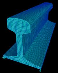
Discretization can provide even great wins. If a problem is amenable to high-order accuracy, a higher order method will unequivocally win over a low-order method. The problem is that most practical problems you can get paid to solve don’t have this property. In almost every case the solution will converge at a first-order accuracy. This is the nature of the world. The knee-jerk response is that this means that high-order methods are not useful. This shows a lack of understanding on what they bring to the table and how they scale. High-order methods produce lower errors than low-order methods even when high-order accuracy cannot be achieved.

As a simple example take a high-order method that delivers half the error of a low order method. To get equivalent results the high-order method would take half the mesh defined by a number of “cell” or “elements” per dimension . If one is interested in time-dependent problems, the number of time steps is usually proportional to . Hence a one-dimensional problem would require degrees of freedom. For equivalent accuracy the high-order method would require cells and one-fourth of the degrees of freedom. It breaks even at four times the cost. In three dimensional time dependent problems, the scaling is and the break-even point is 16 in cost. This is imminently doable. Even larger improvements in accuracy would provide an even more insurmountable advantage.

The counter-point to these methods is their computational cost and complexity. The second issue is their fragility, which can be recast as their robustness or stability in the face of real problems. Still their performance gains are sufficient to amortize the costs given the vast magnitude of the accuracy gains and effective scaling.

An expert is a person who has made all the mistakes that can be made in a very narrow field.

― Niels Bohr

The last issue to touch upon is the need to make algorithms robust, which is just another word for stable. Work on stability of algorithms is simply not happening these days. Part of the consequence is a lack of progress. For example one way to view the lack of ability of multigrid to dominate numerical linear algebra is its lack of robustness (stability). The same thing holds for high-order discretizations, which are typically not as robust or stable as low order ones. As a result low-order methods dominate scientific computing. For algorithms to prosper work on stability and robustness needs to be part of the recipe.

If we knew what it was we were doing, it would not be called research, would it?

― Albert Einstein

Performance is a monotonically sucking function of time. Our current approach to HPC will not help matters, and effectively ignores the ability of algorithms to make things better. So “do we have the right priorities?” and “is this goal (of computing supremacy) important and worthy of achieving?” The answers are an unqualified NO and a qualified YES. The goal of computing dominance and supremacy is certainly worth achieving, but having the fastest computer will absolutely not get us there. It is neither necessary, nor sufficient for success.

This gets to the issue of priorities directly. Our current program is so intellectually bankrupt as to be comical, and reflects a starkly superficial thinking that ignores the sort of facts staring them directly in the face such as the evidence of commercial computing. Computing matters because of how it impacts the real world we live it. This means the applications of computing matter most of all. In the approach to computing taken today the applications are taken completely for granted, and reality is a mere afterthought.

Any sufficiently advanced technology is indistinguishable from magic.

― Arthur C. Clarke

[E]xceptional claims demand exceptional evidence.

What can be asserted without evidence can also be dismissed without evidence.

― Christopher Hitchens

Commercial CFD and mechanics codes are an increasingly big deal. They would have you believe that the only thing people should concern themselves with is the meshing problems, graphical user interfaces, and computer power. The innards of the code with its models and methods are basically in the bag, and no big deal. The quality of the solutions is assured because it’s a solved problem. Input your problem in a point and click manner, mesh it, run it on a big enough computer and point and click visuals, then you’re done.

Marketing is what you do when your product is no good.

― Edwin H. Land

Of course this is not the case, not even close. One might understand why these vendors might prefer to sell their product with this mindset. The truth is that the methods in the codes are old, generally not very good by modern standards. If we had a healthy research agenda for developing improved methods, the methods in the codes would be appalling. On the other hand they are well understood, highly reliable or robust (meaning they will run to completion without undue user intervention). This doesn’t mean that they are correct or accurate. The problem is that they represent a very low bar of success. The codes and the methods utilized by them are far below what might be possible with a healthy computational science program.

Another huge issue is the targeted audience of the users for these codes. If we go back in time we could rely upon the codes being used only by people with PhD’s. Nowadays the codes are targeted at people with Bachelor’s degrees with little or no expertise or interest in numerical methods or advanced models in the context of partial differential equations. As a result, these aspects of the code’s makeup and behavior have been systematically reduced in importance to being practically ignored. Of course, because I work at these very details provides me with the knowledge and evidence that these aspects are paramount in importance. All the meshing, graphics and gee-whiz interface can’t overcome a bad model or method in a code.

Reality is one of the possibilities I cannot afford to ignore

― Leonard Cohen

One way to get to the truth is verification and validation (V&V). While V&V has become an important technical endeavor, it usually is applied more as a buzzword than an actual technical competence. The result is usually a set of activities that have more of the look and feel of V&V than the actual proper practice of V&V. Those marketing the codes tend to trumpet their commitment to V&V while actually espousing the cutting of V&V corners. Part of the problem is that rigorous V&V would in large part undercut many of their marketing premises.

We all die. The goal isn’t to live forever, the goal is to create something that will.

― Chuck Palahniuk

What is truly terrifying about the state of affairs today is that this attitude has gone beyond the commercial code vendors and increasingly defines the attitude at National Labs, and Academia, the place where innovation should be coming from? Money for developing new methods and models has dried up. The emphasis in computational science has shifted to parallel computing and the acquisition of massive new computer platforms.

Reality is that which, when you stop believing in it, doesn’t go away.

― Philip K. Dick

The unifying theme in all of this is that the perception that is being floated is modeling and numerical methods is a solved area of investigation and we simply await a powerful enough computer to unveil the secrets of the universe. This sort of mindset is more appropriate for some sort of cultish religion than science. It is actually antithetical to science, and the result is a lack of real scientific progress.

Don’t try to follow trends. Create them.

― Simon Zingerman

So, what is needed?

• Computational science needs to acknowledge and play by the scientific method. Increasingly, today it does not. It acts on articles of faith and politically correct low risk paths to “progress”.
• We need to cease believing that all our problems will be solved by a faster computer
• The needs of computational science should balance the benefits of models, methods, algorithms, implementation, software and hardware instead of the articles of faith taken today.
• Embrace risks needed for breakthroughs in all of these areas especially models, methods and algorithms, which require creative work and generally need inspired results for progress.
• Acknowledge that the impact of computational science on reality is most greatly improved by modeling improvements. Next in impact are methods and algorithms, which provide greater efficiency. Instead our focus on implementation, software and hardware actually produces less impact on reality.
• Practice V&V with rigor and depth in a way that provides unambiguous evidence that calculations are trustworthy in a well-defined and supportable manner.
• Acknowledge the absolute need for experimental and observational science in providing the window into reality.
• Stop overselling modeling and simulation as an absolute replacement for experiments, and more as a guide for intuition and exploration to be used in association with other scientific methods.

Reality is frequently inaccurate.

― Douglas Adams

A life spent making mistakes is not only more honorable, but more useful than a life spent doing nothing.

― George Bernard Shaw

High performance computing is a hot topic these days. All sorts of promises have been made regarding its transformative potential. Computational modeling is viewed as the cure to the lack of ability to do expensive, dangerous or even illegal experiments. All sorts of benefits are supposed to rain down upon society as a driver of a faster, better and cheaper future. If we were collectively doing everything that should be done these promises might have a chance of coming true, but we’re not and they won’t, unless we start doing things differently.

The Chinese use two brush strokes to write the word ‘crisis.’ One brush stroke stands for danger; the other for opportunity. In a crisis, be aware of the danger–but recognize the opportunity.

― John F. Kennedy

 So, what the hell?

Computing’s ability to deliver on these promises is at risk, ironically due to a lack of risk taking. The scientific computing community seems to have rallied around taking the safe path of looking toward faster computing hardware as the route toward enhanced performance. High payoff activities such as new model or algorithm development are also risky and likely to fail with high probability. The relatively small number of successful projects in these areas result in massive payoffs in terms of performance.

Despite a strong historical track record of providing greater benefits for computational simulation than hardware efforts to improve modeling, methods and algorithms are starved for support. This will kill the proverbial goose that is about to lay a golden egg. We are figuratively strangling the baby in the crib by failing to feed the core of creative value in simulation. We have prematurely declared that computational simulation is mature and ready for prime time. In the process we are stunting its growth and throwing money away on developing monstrous computers to feed computational power to a “petulant teen”. Instead we need to develop the field of simulation further and make some key steps toward providing society with a mature and vibrant scientific enterprise. Policy makers have defined a future where the only thing that determines computational simulation capability to be the computing power of the computer it runs on.

This mindset has allowed the focus to shift almost in its entirety toward computing hardware. Growth in the performance of computing power is commonly used as an advertisement for the access and ease of utilizing computational modeling. An increasing number of options exist for simply buying simulation capability in the form of computational codes. The user interfaces for the codes allows relatively broad access to modeling and definitely takes the capability out of the hands of the experts. For those selling capability this democratization is a benefit because it increases the size of the market. Describing this area as a mature, solved problem is another marketing benefit.

The question of whether this is a good thing still needs to be asked. How true are these marketing pitches?

It is relatively easy to solve problems today. Computer power allows the definition of seemingly highly detailed models and fine computational grid as well as stunning visual representations. All of these characteristics provide users with the feeling of simulation quality. The rise of verification and validation should allow the users to actually determine whether these feelings are justified. Generally V&V undermines ones belief in how good results are. On the other hand people like to feel that their analysis is good. This means that much of the negative evidence is discounted or even dismissed when conducting V&V. The real effect of the slipshod V&V is to avoid the sort of deep feedback that the quality of results should have on the codes.

When you fail, that is when you get closer to success.

― Stephen Richards

At this juncture it’s important to talk about current codes and the models and methods contained in them. The core of the philosophy of code based modeling goes all the way back into the 1960’s and has not changed much since. This is a problem. In many cases the methods used in the codes to solve the models are nearly as old. In many cases the methods were largely perfected during the 1970’s and 1980’s. Little or no effort is presently being put forth to advance the solutions techniques. In summary most effort is being applied to simply implementing the existing solution techniques on the next generation of computers.

Remember the two benefits of failure. First, if you do fail, you learn what doesn’t work; and second, the failure gives you the opportunity to try a new approach.

― Roger Von Ouch

Almost certainly the models themselves are even more deeply ensconced and effectively permanent. No one even considers changing the governing equations being solved. Models of course have a couple of components, the basic governing equations are generally quite classical, and their closure is the part that slowly evolves. These equations were the product of 17^th-19^th Century science and philosophical mindset that should being questioned if science itself were healthy. If one thinks about the approach we take today, the ability to resolve new length and time scales it has changed monumentally. We should be able to solve vastly nonlinear systems of equations (we really can’t in a practical robust manner). Is it even appropriate to have the same equations? Or should the nature of the equations change as a function of the characteristic scales of resolution. Closure modeling evolves more readily, but only within the philosophical confines defined by the governing equations. Again, we are woefully static, and the lack of risk taking is undermining any promise for actual promise.

Take the practice of how material properties are applied to a problem as a key point. The standard way to apply material properties is to “paint” the properties into regions containing a material. For example if aluminum exists in the problem, a model defines the properties with its response to forces. The aluminum is defined, as being the same everywhere there is aluminum. As the scale size gets smaller aluminum (or any material) gets less and less homogeneous. There begins to be significant differences in the structure typically defined by the grain structure of the material and any imperfections. The model is systematically ignoring these heterogeneous features. Usually their collective effects are incorporated in an average way in the model, but the local effects of these details are ignored. Modern application questions are more and more focused upon the sort of unusual effects that happen due to these local defects.

Experimental observations are only experience carefully planned in advance, and designed to form a secure basis of new knowledge.

― Sir Ronald Fisher

Let’s be perfectly blunt and clear about the topic of modeling. The model we solve in simulation is the single most important and valuable aspect of a computation. A change in the model that opens new physical vistas is more valuable than any computer including one with limitless power. A computer is no better than the model it solves. This point of view is utterly lost today.

More dangerously we are continuing to write codes for the future in the same manner today. In other words we have had the same philosophy in computational modeling for the last 50 years or more. The same governing equations and closure philosophy are being used today. How much longer will be continue to do the same thing? I believe we should have changed a while ago. We can begin to study the impact of material and solution heterogeneity already, but the models and methods to do so are not being given any priority.

The reason is that it would be disruptive and risky. It would require changing our codes and practices significantly. It would undermine the narrative of computer power as the tonic for what ails us. It would be a messy and difficult path. It would also be consistent with the scientific method instead of following a poorly thought through intellectually empty article of faith. Because risk taking is so antithetical today this path has been avoided.

Our most significant opportunities will be found in times of greatest difficulty.

― Thomas S. Monson

The investments in faster computers are valuable and beneficial, but only if these investments are balanced with other investments. Modeling is the aspect of computation that is closest to reality and holds the greatest leverage and value. Methods for solving models and associated algorithms are next closest and have the next highest leverage. Neither of these areas is being invested in at a healthy level. Implementing these algorithms and models is next most important. Here there is a little more effort because existing models need to work on the computers. The two areas with the highest level of effort are system software and hardware. Ironically these two areas have the least amount of value in terms of effecting reality. No one in a position of power seems to recognize how antithetical to progress this state of affairs is.

Sometimes it’s the mistakes that turn out to be the best parts of life

― Carrie Ryan

Hypocrites get offended by the truth.

― Jess C. Scott

The overall quality of computational modeling depends on a lot of things and one very big one isn’t generally acknowledged, whoever is using the code. How much does it matter? A lot, much more than almost anyone would admit and the effect becomes greater as problem complexity grows.

The most important property of a program is whether it accomplishes the intention of its user.

― C.A.R. Hoare

The computer, the code, the computational resolution (i.e., mesh), the data, the models, and the theory all get acute and continuous attention from verification and validation. When the human element in quality is raised as an issue, people become immensely defensive. At the same time it is generally acknowledged by knowledgeable people that the impact of the user of the code (or modeler) is huge. In many cases it may be the single greatest source of uncertainty.

We don’t see things as they are, we see them as we are.

― Anaïs Nin

This isn’t a matter of simple mistakes made in the modeling process; this is associated with reasonable choices made in representing complex problems. Different modelers make different decisions about dealing with circumstances and representing all the “gray” area. In many cases these choices live in the space where variability in results should be. For example the boundary or initial conditions are common sources of the changes. Reality is rarely fully reproducible and details that are generally fuzzy result are subtle changes in outcomes. In this space, the user of a code can different, but equally reasonable choices about how to model a problem. These can result in very large changes in results.

Despite this the whole area of uncertainty quantification of this effect is largely missing. This is because it is such an uncomfortable source of variation in results. Only a few areas readily acknowledge or account for this such as nuclear reactor safety work, the Sandia “Fracture Challenge” and a handful of other isolated cases. It is something that needs much greater attention, but only if we are courageous enough to attack the problem.

It’s funny how humans can wrap their mind around things and fit them into their version of reality.

― Rick Riordan

The capacity to acknowledge this effect and measure it is largely resisted by the community. We are supposed to live in an age where everything is automatic and the computer will magically unveil the truths of the universe to us. This is magical thinking, but the commonly accepted dogma of modernity. Instead the core of value is fundamentally connected to the human element, and this truth seems to beyond our ability to admit.

We do not need magic to transform our world. We carry all of the power we need inside ourselves already.

― J.K. Rowling

Physics is becoming so unbelievably complex that it is taking longer and longer to train a physicist. It is taking so long, in fact, to train a physicist to the place where he understands the nature of physical problems that he is already too old to solve them.

— Eugene Paul Wigner

The past decade has seen the rise of commercial modeling and simulation tools with seemingly great capabilities. Computer power has opened vistas of simulation to the common engineer and scientist. Advances in other related technologies like visualization have provided an increasingly “turn-key” experience to users who can do seemingly credible cutting-edge work on their laptops. These advances also carry with them some real dangers most acutely summarized as a “black box” mentality toward the entire modeling and simulation enterprise.

artificial intelligence is no match for natural stupidity

—Albert Einstein

Black box thinking causes problems because people get answers without understanding how those answers are arrived at. When problems are simple and straightforward this can work, but as soon as the problems become difficult issues arise. The models and methods in a code can do funny things that only make sense knowing the inner workings of the code. The black box point of view usually comes with too much trust of what the code is doing. This can cause people to accept solutions that really should have been subjected to far more scrutiny.

The missing element in the black box mentality is the sense of collaboration needed to make modeling and simulation work. The best work is always collaborative including elements of computation and modeling, but also experiments, mathematics and its practical applications. This degree of multi-disciplinary work is strongly discouraged today. Ironically, the demands of cost accounting often work steadfastly to undermine the quality of work by dividing people and their efforts into tidy bins. The drive to make everything accountable discourages the ability to conduct work in the best way possible. Instead our current system of management encourages the black box mentality.

Another force for pushing black box thinking is education. Students now run codes whose interface is easy enough to bear some resemblance to video games. Of course with a generation of scientists and engineers raised on video games this could be quite powerful. At the same time the details of the codes are not generally emphasized, and instead they tend to be viewed as black boxes. In classes when the details of the codes are unveiled, eyes glaze over and it becomes clear that the only thing they are really interested in is getting results, not knowing how the results were arrived at.

One way this current trend is being blunted is the adoption of verification and validation (V&V) in modeling and simulation. V&V encourages a distinct multidisciplinary point-of-view in its execution particularly when coupled to uncertainty quantification. To do V&V correctly requires a significant amount of deep knowledge of many technical areas. This is really difficult. Instead of engaging deeply in the technical work necessary for good V&V is simply beyond the capacity of most people’s capabilities and tolerance for effort. People paying for modeling and simulation for the most part are unwilling to pay for good V&V. They would rather have V&V that is cheap and fools people into confidence.

Computers are incredibly fast, accurate, and stupid: humans are incredibly slow, inaccurate and brilliant; together they are powerful beyond imagination.

― Albert Einstein

Two elements are leading to this problem. No one is willing to pay for high-quality technical work either the development or use of simulation codes. Additionally no one is willing to pay for the developers of the code and the users to work together. The funding, environment and tolerance to support the sort of multi-disciplinary activities that produce good modeling and simulation (and by virtue of that goo V&V) is shrinking with each passing year. Developing professionals who do this sort of work well is really expensive and time-consuming. When the edict is to simply crank out calculations with a turnkey technology, the appetite for running issues to ground necessary for quality simply doesn’t exist.

A couple of issues have really “poisoned the well” of modeling and simulation. The belief is that the technology is completely trustworthy and mature enough for novices to use is an illusion. Commercial codes are certainly useful, but need to be used with skill and care by curious, doubtful users. These codes often place a serious premium on robustness over accuracy, and cut lots of corners to keep their users happy. A happy user is usually first and foremost someone with a completed calculation regardless of the credibility of that calculation. We also believe that everything is deeply enabled by almost limitless computing power.

Think? Why think! We have computers to do that for us.

— Jean Rostand

Computing power doesn’t relieve us of the responsibility to think about what we are doing. We should stop believing that the computational tools can be used like magic, black magic in black boxes that we don’t understand. If you don’t understand how you got your answers, you probably shouldn’t trust that answer until you do.

A computer lets you make more mistakes faster than any other invention with the possible exceptions of handguns and Tequila.

— Mitch Ratcliffe

The reasonable man adapts himself to the world: the unreasonable one persists in trying to adapt the world to himself. Therefore all progress depends on the unreasonable man.

― George Bernard Shaw

We appear to be living in a golden age of progress. I’ve come increasingly to the view that this is false. We are living in an age that is enjoying the fruits of a golden age and following the inertia of a scientific golden age. The forces powering the “progress” we enjoy are not being returned to our future generations. So, what are we going to do when we run out of the gains made by our fore bearers?

Progress is a tremendous bounty to all. We can all benefit from wealth, longer and healthier lives, greater knowledge and general well-being. The forces arrayed against progress are small-minded and petty. For some reason the small-minded and petty interests have swamped forces for good and beneficial efforts. Another way of saying this is the forces of the status quo are working to keep change from happening. The status quo forces are powerful and well-served by keeping things as they are. Income inequality and conservatism are closely related because progress and change favors those who benefit from change. The people at the top favor keeping things just as they are.

 Those who do not move, do not notice their chains.

― Rosa Luxemburg

Most of the technology that powers today’s world was actually developed a long time ago. Today the technology is simply being brought to “market”. Technology at a commercial level has a very long lead-time. The breakthroughs in science that surrounded the effort fighting the Cold War provide the basis of most of our modern society. Cell phones, computers, cars, planes, etc. are all associated with the science done decades ago. The road to commercial success is long and today’s economic supremacy is based on yesterday’s investments.

Without deviation from the norm, progress is not possible.

― Frank Zappa

Since the amount of long-term investment today is virtually zero, we can expect virtually zero return down the road. We aren’t effectively putting resources into basic or applied research much as we aren’t keeping up with roads and bridges. Our low-risk approach to everything is sapping the vitality from research. We compound this by failing to keep our 20^th Century infrastructure healthy, and completely failing to provide a 21^st Century one (just look at our pathetic internet speeds). Even where we spend lots on money on things like science little investment is happening because of the dysfunctional system. One of the big things hurting any march toward progress is the inability to take risks. Because failure is so heavily penalized, people won’t take the risks necessary for success. If you can’t fail, you can’t succeed either. It is an utterly viscous cycle that highlights the nearly complete lack of leadership. The lack of action by National leadership is simply destroying the quality of our future.

Restlessness is discontent — and discontent is the first necessity of progress. Show me a thoroughly satisfied man — and I will show you a failure.

― Thomas A. Edison

Take high performance computing as an example. In many respects the breakthroughs in algorithms have been as important as the computers themselves. Lack of risk taking has highlighted the computers as the source of progress because of Moore’s law. Algorithmic work is more speculative and hence risky. Payoffs are huge, but infrequent and thus risky. Effort might be expended that yields nothing at all. There shouldn’t be anything wrong with that! Because they are risky they are not favored.

We can only see a short distance ahead, but we can seeplenty there that needs to be done.

― Alan Turing

A secondary impact of the focus on computers is that the newer computing approaches are really hard to use. It is a very hard problem to simply get the old algorithmic approaches to work at all. With so much effort going into implementation as well as being siphoned from new algorithmic research, the end product is stagnation. Numerical linear algebra is a good example of this terrible cycle in action. The last real algorithm breakthrough is multigrid about 30 years ago. Since then work has focused on making the algorithms work on massively parallel computers.

Progress always involves risk; you can’t steal second base and keep your foot on first

― F.W. Dupee

The net result is lack of progress. Our leaders are seemingly oblivious to the depth of the problem. They are too caught up in trying to justify the funding for the path they are already taking. The damage done to long-term progress is accumulating with each passing year. Our leadership will not put significant resources into things that pay off far into the future (what good will that do them?). We have missed a number of potentially massive breakthroughs chasing progress from computers alone. The lack of perspective and balance in the course for progress shows a stunning lack of knowledge for the history of computing. The entire strategy is remarkably bankrupt philosophically. It is playing to the lowest intellectual denominator. An analogy that does the strategy too much justice would compare this to rating cars solely on the basis of horsepower.

A person who makes few mistakes makes little progress.

― Bryant McGill

The end product of our current strategy will ultimately starve the World of an avenue for progress. Our children will be those most acutely impacted by our mistakes. Of course we could chart another path that balanced computing emphasis with algorithms, methods and models. Improvements in our grasp of physics and engineering should probably be in the driver’s seat. This would require a significant shift in the focus, but the benefits would be profound.

One of the most moral acts is to create a space in which life can move forward.

― Robert M. Pirsig

What we lack is the concept of stewardship to combine with leadership. Our leaders are stewards of the future, or they should be. Instead they focus almost exclusively on the present with the future left to fend for itself.

Human progress is neither automatic nor inevitable… Every step toward the goal of justice requires sacrifice, suffering, and struggle; the tireless exertions and passionate concern of dedicated individuals.

― Martin Luther King Jr.

Maturity, one discovers, has everything to do with the acceptance of ‘not knowing.

― Mark Z. Danielewski

Uncertainty quantification is a hot topic. It is growing in importance and practice, but people should be realistic about it. It is always incomplete. We hope that we have captured the major forms of uncertainty, but the truth is that our assumptions about simulation blind us to some degree. This is the impact of “unknown knowns” the assumptions we make without knowing we are making them. In most cases our uncertainty estimates are held hostage to the tools at our disposal. One way of thinking about this looks at codes as the tools, but the issue is far deeper actually being the basic foundation we base of modeling of reality upon.

… Nature almost surely operates by combining chance with necessity, randomness with determinism…

― Eric Chaisson

One of the really uplifting trends in computational simulations is the focus on uncertainty estimation as part of the solution. This work is serving the demands of decision makers who increasingly depend on simulation. The practice allows simulations to come with a multi-faceted “error” bar. Just like the simulations themselves the uncertainty is going to be imperfect, and typically far more imperfect than the simulations themselves. It is important to recognize the nature of imperfection and incompleteness inherent in uncertainty quantification. The uncertainty itself comes from a number of sources, some interchangeable.

Sometimes the hardest pieces of a puzzle to assemble, are the ones missing from the box.

― Dixie Waters

Let’s explore the basic types of uncertainty we study:

Epistemic: This is the uncertainty that comes from lack of knowledge. This could be associated with our imperfect modeling of systems and phenomena, or materials. It could come from our lack of knowledge regarding the precise composition and configuration of the systems we study. It could come from the lack of modeling for physical processes or features of a system (e.g., neglecting radiation transport, or relativistic effects). Epistemic uncertainty is the dominant form of uncertainty reported because tools exist to estimate it, and it treats simulation codes like “black boxes”.

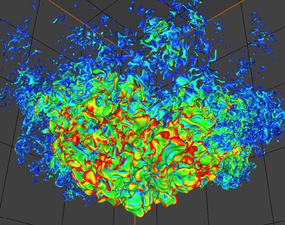
Aleatory: This is uncertainty due to the variability of phenomena. This is the weather. The archetype of variability is turbulence, but also think about the detailed composition of every single device. They are all different in some small degree never mind their history after being built. To some extent aleatory uncertainty is associated with a breakdown of continuum hypothesis and is distinctly scale dependent. As things are simulated at smaller scales different assumptions must be made. Systems will vary at a range of length and time scales, and as scales come into focus their variation must be simulated. One might argue that this is epistemic, in that if we could measure things precisely enough then it could be precisely simulated (given the right equations, constitutive equation and boundary conditions). This point of view is rational and constructive only to a small degree. For many systems of interest chaos reigns and measurements will never be precise enough to matter. By and large this form of uncertainty is simply ignored because simulations can’t provide information.

Numerical: Simulations involve taking a “continuous” system and cutting them up into discrete pieces. Insofar as the equations describe reality the solutions should approach a correct solution as these pieces get more numerous (and smaller). This is the essence of mesh refinement. Computational simulation is predicated upon this notion to an increasingly ridiculous degree. Regardless of the viability of the notion, the approximations made numerically are a source of error to be included in any errorbar. Too often these errors are ignored, wrongly assumed to be small, or incorrectly estimated. There is no excuse for this today.

Users: the last sources of uncertainty examined are the people who use codes and construct models to be solved. As problem complexity grows the decisions in modeling become more subtle and prone to variability. Quite often modelers of equal skill will come up with distinctly different answers or uncertainties. Usually a problem is only modeled once, so this form of uncertainty (or the requisite uncertainty on the uncertainty) is completely hidden from view. Unless there is an understanding of how the problem definition and solution choices impact the solution, the uncertainty will be unquantified. Knowledge of this uncertainty is almost always larger for complex problems where it is less likely for the simulations to be conducted by independent teams. Studies have shown this to be as large or larger than other sources! Almost the only place this has received any systematic attention is nuclear reactor safety analysis.

As far as the laws of mathematics refer to reality, they are not certain; and as far as they are certain, they do not refer to reality.

― Albert Einstein

One has to acknowledge that the line between epistemic and aleatory is necessarily fuzzy. In a sense the balance is tipped toward epistemic because of the tools exist to study it. At some level this is a completely unsatisfactory state of affairs. Some features of systems arise from the random behavior of the constituent parts of the system. Systems and their circumstances are just a little different, and these differences yield differences (sometimes slight) in the response. Sometimes these small differences create huge changes in the outcomes. It is these huge changes that drive a great deal of worry in decision-making. Addressing these issue is a huge challenge for computational modeling and simulation; a challenge that we simply aren’t addressing at all today.

Why?

The assumption of an absolute determinism is the essential foundation of every scientific enquiry.

― Max Planck

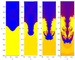A large part of the reason for failing to address these matters is the implicit, but slavish devotion to determinism. Simulations are almost always viewed as the solution to a deterministic problem. This means there is AN answer. Answers are almost never sought in the sense of a probability distribution. Even probabilistic methods like Monte Carlo are trying to approach the deterministic solution. Reality is almost never AN answer and almost always a distribution. What we end up solving is the mean expected response of a system to the average circumstance. What is actually observed is a distribution of responses to a distribution of circumstances. Often the real question to answer in any study (with or without simulation) is what’s the worse that can reasonably happen? A level of confidence that says 95% or 99% of the responses will be less than some bad level usually defines the desired result. This sort of question is best thought of as aleatory, and our current simulation capability doesn’t begin to address it.

When your ideas shatter established thought, expect blowback.

― Tim Fargo

The key aspect of this entire problem is a slavish devotion to determinism in modeling. Almost every modeling discipline sees the solution being sought as being utterly deterministic. This is logical if the conditions being modeled are known with exceeding precision. The problem is that such precision is virtually impossible for any circumstance. This is the core of the problem with simulating the aleatory uncertainty that so frequently remains untreated. It is almost completely ignored by a host of fundamental assumption in modeling that is inherited by simulations. These assumptions are holding back real progress in a host of fields of major importance.

Finally we must combine all these uncertainties to get our putative “error bar”. There are a number of ways to go about this combination with varying properties. The most popular knee-jerk approach is to use the root mean square of the contributions (square root of the sum of the squares). The sum of the absolute values would be a better and safer choice, since it is always larger (hence more conservative) than the sum of squares. If you’re feeling cavalier and want to play it dangerous, just use the largest uncertainty. Each of these choices is related to probabilistic assumptions, which in the case of sum of squares is assuming a normal distribution.

It is impossible to trap modern physics into predicting anything with perfect determinism because it deals with probabilities from the outset.

― Arthur Stanley Eddington

One of the most pernicious and deepening issues associated with uncertainty quantification is “black box” thinking. In many cases the simulation code is viewed as being a black box where the user knows very about its workings beyond a purely functional level. This often results in generic and generally uninformed decisions being made on uncertainty. The expectations of the models and numericalmethods are understood only superficially, and this results in a superficial uncertainty estimate. Often the black box thinking extends to the tool used to get uncertainty too. We then get the result from a superposition of two black boxes. Not a lot light bets shed on reality in the process. Numerical errors are ignored, or simply misdiagnosed. Black box users often simply do a mesh sensitivity study, and assume that small changes under mesh variation are indicative of convergence and small errors. They may or may not be such evidence. Without doing a more formal analysis this sort of conclusion is not justified. If code and problem is not converging, the small changes may be indicative of very large numerical errors or even divergence and a complete lack of control.

Whether or not it is clear to you,

no doubt the universe is unfolding

as it should.

― Max Ehrmann

The answer to this problem is deceptively simple make things “white box” testing. The problem is that making our black boxes into white boxes is far from simple. Perhaps the hardest thing about this is having people doing the modeling and simulation with sufficient expertise to treat the tools as white boxes. A more reasonable step forward is for people to simply realize the dangers inherent in black box testing mentality.

Science is a way of thinking much more than it is a body of knowledge.

― Carl Sagan

In many respects uncertainty quantification is in its infancy. The techniques are immature and terribly incomplete. Beyond this character, we are deeply tied to modeling philosophies that hold us back from progress. The whole field needs to mature and throw off the shackles imposed by the legacy of Newton and the entire rule of determinism that still holds much of science under its spell.

The riskiest thing we can do is just maintain the status quo.

― Bob Iger

When you stop growing you start dying.

― William S. Burroughs

Moore’s law isn’t a law, but rather an empirical observation that has held sway for far longer than could have been imagined fifty years ago. In some way shape or form, Moore’s law has provided a powerful narrative for the triumph of computer technology in our modern World. For a while it seemed almost magical in its gift of massive growth in computing power over the scant passage of time. Like all good things, it will come to an end, and soon if not already.

Its death is an inevitable event, and those who have become overly reliant upon its bounty are quaking in their shoes. For the vast majority of society Moore’s law has already faded away. Our phones and personal computers no longer become obsolete due to raw performance every two or three years. Today obsolescence comes from software, or advances in the hardware’s capability to be miserly with power (longer battery life on your phone!). Scientific computing remains fully in the grip of Moore’s law fever! Much in the same way that death is ugly and expensive for people, the death of Moore’s law for scientific computing will be the same. 

Nothing can last forever. There isn’t any memory, no matter how intense, that doesn’t fade out at last.

― Juan Rulfo

One of the most pernicious and difficult problems with health care is end of life treatment (especially in the USA). An enormous portion of the money spent on a person’s health care is focused on the end of life (25% or more). Quite often these expenses actually harm people and reduce their quality of life. Rarely do the expensive treatments have a significant impact on the outcomes, yet we spend the money because death is so scary and final. The question I’m asking is whether we are about to do exactly the same thing with Moore’s law in scientific computing?

Yes.

 Moore’s law is certainly going to end. In practical terms it may already be dead with it holding only in the case of completely impractical stunt calculations. If one looks at the scaling of calculations with modest practical importance such as the direct numerical simulation of turbulence the conclusion is that Moore’s law has passed away. The growth in capability has simply fallen dramatically off the pace we would expect from Moore’s law. If one looks at the rhetoric in the national exascale initiative, the opposite case is made. We are going forward guns blazing. The issue is just the same as end of life care for people, is the cost worth the benefit?

Its hard to die. Harder to live

― Dan Simmons

The computers that are envisioned for the next decade are monstrosities. They are impractical and sure to be nearly impossible to use. They will be unreliable. They will be horrors to program. Almost everything about these computers is utterly repulsive to contemplate. Most of all these computers will be immense challenges to conduct any practical work on. Despite all these obvious problems we are going to spend vast sums of money acquiring these computers. All of this stupidity will be in pursuit of a vacuous goal of the fastest computer. It will only be the fastest in terms of a meaningless benchmark too.

Real dishes break. That’s how you know they’re real.

― Marty Rubin

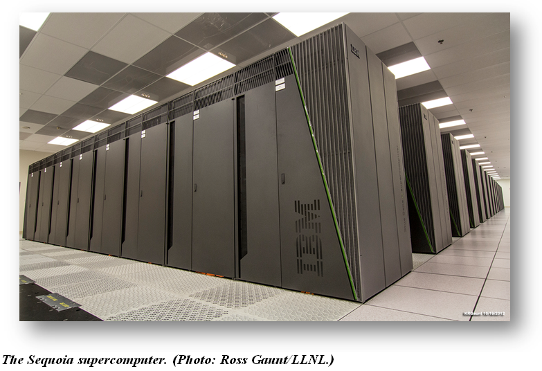
For those of us doing real practical work on computers this program is a disaster. Even doing the same things we do today will be harder and more expensive. It is likely that the practical work will get harder to complete and more difficult to be sure of. Real gains in throughput are likely to be far less than the reported gains in performance attributed to the new computers too. In sum the program will almost certainly be a massive waste of money. The plan is for most of the money going to the hardware and the hardware vendors (should I think corporate welfare?). All of this will be done to squeeze another 7 to 10 years of life out of Moore’s law even though the patient is metaphorically in a coma already.

The bottom line is that the people running our scientific computing programs think that they can sell hardware. The parts of scientific computing where the value comes from can’t be persuasively sold. As a result modeling, methods, algorithms and all the things that make scientific computing actually worth doing are starved for support. Worse yet, the support they do receive is completely swallowed up by trying to simply make current models, methods and algorithms work on the monstrous computers we are buying.

What would be a better path for us to take?

Let Moore’s law die, hold a wake and chart a new path. Instead of building computers to be fast, build them to be useful and easy to use. Start focusing some real energy on modeling, methods and algorithms. Instead of solving the problems we had in scientific computing from 1990, start working toward methodologies that solve tomorrow’s problems. All the things we are ignoring have the capacity to add much more value than our present path.

For nothing is evil in the beginning.

― J.R.R. Tolkien

The irony of this entire saga is that computing could mean so much more to society if we valued the computers themselves less. If we simply embraced the evitable death of Moore’s law we could open the doors to innovation in computing instead of killing it in pursuit of a foolish and wasteful extension of its hold.

The most optimistic part of life is its mortality… God is a real genius.

― Rana Zahid Iqbal

Your assumptions are your windows on the world. Scrub them off every once in a while, or the light won’t come in.

― Isaac Asimov

If someone gives you some data and asks you to fit a function that “models” the data, many of you know the intuitive answer, “least squares”. This is the obvious, simple choice, and perhaps, not surprisingly, not the best answer. How bad this choice may be depends on the situation? One way to do better is to recognize the situations where the solution via least squares may be problematic, and produce an undue influence on the results.

Most of our assumptions have outlived their uselessness.

― Marshall McLuhan

To say that this problem is really important to the conduct of science is a vast understatement. The reduction of data is quite often posed in terms a simple model (linear terms in important parameters) and solved via least squares. The data is often precious, or very expensive to measure. Given the importance of data in science it is ironic that we should so often take the final hurtle so cavalierly and apply such a crude manner to analyze it as least squares. More properly we don’t consider the consequences of such an important choice, usually it isn’t even thought of as a choice.

That’s the way progress works: the more we build up these vast repertoires of scientific and technological understanding, the more we conceal them.

― Steven Johnson

The key to this is awakening to the assumptions made in least squares. The key assumption is the nature of the assumed errors in fit, which is normally distributed (or Gaussian) statistics for least squares. If you know this to be true then least squares is the right choice. If this is not true, then you might be introducing a rather significant assumption (a known unknown if you will) into your fit. In other words your results will be based upon an assumption you don’t even know that you made.

If your data and model match quite well and the deviations are small, it also may not matter (much). This doesn’t make least squares a good choice, just not a damagingone. If the deviations are large or some of your data might be corrupt (i.e., outliers), the choice of least squares can be catastrophic. The corrupt data may have a completely overwhelming impact on the fit. There are a number of methods for dealing with outliers in least squares, and in my opinion none of them good.

 The difficulty lies not so much in developing new ideas as in escaping from old ones.

― John Maynard Keynes

Fortunately there are existing methods that are free from these pathologies. For example the least median deviation fit can deal with corrupt data easily. It naturally excludes outliers from the fit because of a different underlying model. Where least squares are the solution of a minimization problem in the energy or L2 norm, the least median deviation uses the L1 norm. The problem is that the fitting algorithm is inherently nonlinear, and generally not included in most software.

I suppose it is tempting, if the only tool you have is a hammer, to treat everything as if it were a nail.

― Abraham Maslow

One of the problems is that least squares are virtually knee-jerk in its application. It is contained in standard software such as Microsoft Excel and can be applied with almost no thought. If you have to write your own curve-fitting program by far the simplest approach is to use least squares. It can often produce a linear system of equations to solve where alternatives are invariably nonlinear. The key point is to realize that this convenience has a consequence. If your data reduction is important, it might be a good idea to think about what you ought to do a bit more.

Duh.

The explanation requiring the fewest assumptions is most likely to be correct.

― William of Ockham

Reviews are for readers, not writers. If I get a bad one, I shrug it off. If I get a good one, I don’t believe it
― William Meikle

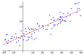
A week ago I received bad news, the review for a paper were back. One might think that getting a review back would be good, but it rarely is. These reviews are too often a horrible soul-crushing experience. In this case I had reports from two reviewers, and one of them delivered the ego thrashing I’ve come to fear.

 I’ve found the best way to revise your own work is to pretend that somebody else wrote it and then to rip the living shit out of it.

― Don Roff

In total the two reviews were generally consistent on the details of the paper, and the sorts of suggestions for bringing the paper into the condition needed to allow publication. The difference was the tone of the reviews. One of the reviews was completely constructive and detailed in its critique. Each and every critique was offered in a positive light even when the error was pure carelessness.

The other review couldn’t be more different in tone. From the outset it felt like an attack on me. It took me until several days until I could read it in a manner that allowed me to take constructive action. For example including a comment that says “the writing is terrible” is basically an attack on the authors (yes it feels personal). This could be stated much more effectively, “I believe that you have something important to say here, but the ideas do not come across clearly.” Both things say the same thing, but one of them invites a positive and constructive response. I invite the readers to endeavor to write your own reviews in a manner to invite authors to improve. One of my co-authors who has a somewhat more unbiased eye noted that the referee’s report seemed a bit defensive.

So now I’m taking the path of revising the paper. A visceral report makes this much more difficult to accomplish. The constructive review is relatively easy to accommodate, and makes for a good blueprint for progress. The nasty review is much harder to employ in the same fashion. I feel that I’m finally on the path to do this, but it could have been much easier. There is nothing wrong with being critical, but the way its done matters a lot.

That’s the magic of revisions – every cut is necessary, and every cut hurts, but something new always grows.

― Kelly Barnhill

Just for the record the paper is titled “Robust Verification Analysis” by myself, Jim Kamm (Los Alamos), Walt Witkowski and Tim Wildey (Sandia), it was submitted to the Journal of Computational Physics. As part of the revision I’ve taken the liberty of rewriting the abstract:

We introduce a new methodology for inferring the accuracy of computational simulations through the practice of solution verification. Our methodology is well suited to both well- and ill-behaved sequences of simulations. Our approach to the analysis of these sequences of simulations incorporates expert judgment into the process directly via a powerful optimization framework, and the application of robust statistics. The expert judgment is systematically applied as constraints to the analysis, and together with the robust statistics guards against over-emphasis on anomalous analysis results. We have named our methodology Robust Verification Analysis.

The practice of verification is a key aspect for determining the correctness of computer codes and their respective computational simulations. In practice verification is conducted through repeating simulations with varying discrete resolution and conducting a systematic analysis of the results. The accuracy of the calculation is computed directly against an exact solution, or inferred by the behavior of the sequence of calculations.

Nonlinear regression is a standard approach to producing the analysis necessary for verification results. We note that nonlinear regression is equivalent to solving a nonlinear optimization problem. Our methodology is based on utilizing multiple constrained optimization problems to solve the verification model in a manner that varies the solutions underlying assumptions. Constraints applied in the solution can include expert judgment regarding convergence rates (bounds and expectations) as well as bounding values for physical quantities (e.g., positivity of energy or density). This approach then produces a number of error models, which are then analyzed through robust statistical techniques (median instead of mean statistics).

This provides self-contained, data driven error estimation including uncertainties for both the solution and order of convergence. Our method will produce high quality results for the well-behaved cases consistent with existing practice. The methodology will also produce reliable results for ill-behaved circumstance. We demonstrate the method and compare the results with standard approaches used for both code and solution verification on well-behaved and more challenging simulations. We pay particular attention to the case where few calculations are available and these calculations are conducted on coarse meshes. These are compared to analytical solutions, or calculations on highly refined meshes.

Here is abstract from the the original submission:

Code and solution verification are key aspects for determining the quality of computer codes and their respective computational simulations. We introduce a verification method that can produce quality results more generally with less well-behaved calculations. We have named this methodology Robust Verification Analysis. Nonlinear regression is a standard approach to producing the analysis necessary for verification results. Nonlinear regression is equivalent to solving a nonlinear optimization problem. We base our methodology on utilizing multiple constrained optimizations to solve the verification model. Constraints can include expert judgment regarding convergence rates and bounding values for physical quantities. This approach then produces a number of error models, which are then analyzed through robust statistical techniques (e.g., median instead of mean statistics). This provides self-contained, data driven error estimation including uncertainties for both the solution and order of convergence. Our method will produce high quality results for the well-behaved cases consistent with existing practice as well. We demonstrate the method and compare the results with standard approaches used for both code and solution verification on well-behaved and challenging data sets.

 There is a saying: Genius is perseverance. While genius does not consist entirely of editing, without editing it’s pretty useless.

― Susan Bell

When you print out your manuscript and read it, marking up with a pen, it sometimes feels like a criminal returning to the scene of a crime.
― Don Roff