Progress is discovering what you can do without.

― Marty Rubin

Note: WordPress LaTeX woes continue so equations that wouldn’t parse are separated by “$” in the TeX “code”.

After last week’s orgy of words I was a bit more restrained this week, after all I am on vacation! It’s a topic that means a lot to me and actually represents a fun topic, so I’m continuing the thematic direction. Go figure! Still some more thoughts on the general recent theme are presented where improvements would mean much more to computational science than a bunch of expensive, hard to use, energy wasting, hard-to-impossible to program computers; Alternatively, improvements in methods that would make those precious computers radically more useful! None of the press regarding “exascale” computing acknowledges that supercomputing is an intrinsically holistic endeavor where the models, methods and algorithmic advances do far more to empower the future than any hardware investments.

Off the soapbox, and on to the chalkboard!

I’ve been advancing the theme of methods for improving the solution of hyperbolic PDEs for several weeks now. At the end of the last post I posited the proposition that looking to produce high order accurate approximation wasn’t always the best idea. Quite often we must content with solutions that are very under-resolved and rough in character. Experience seems to dictate that this eventuality is so important that it should always be present in the method’s design. One of the issues with the ENO and WENO methods is the absence of these ideas from high-order methods, which may be limiting their utility for broad use. Under appropriate conditions abandoning the pursuit of accuracy may be the advisable thing to do. From our experience with first generation monotonicity-preserving methods we can see that under the conditions where accuracy cannot be maintained, the discrete conditions are incredibly useful and powerful. Perhaps there is a route to improvement in methods that may use this experience productively. Limiters seem to endow the methods with a greater and stronger sense of nonlinear stability (i.e., robustness) to the extent of allowing one to use unstable approximations locally in a completely stable, robust manner.

The first thing to do is review the relations for providing monotonicity-preserving methods that can be easily stated by using TVD theory. This was discussed last week. First, the key fact that upwind differencing is a positive scheme is a foundation for things, $ U(j,n+1) = U(j,n) – \nu \left[ U(j,n) – U(j-1,n) \right] $ where is the CFL number. Next, apply this basic thought process to second-order extension (or a high-order extension more generally), . Plugging this into our update equation, $ U(j,n+1) = U(j,n) – \nu \left[ U(j+1/2,n) – U(j-1/2,n) \right] $ can produce conditions on limiters for . These are functional relationships defined by dividing the slope by the upwind difference on the mesh. These produce the famous diagrams introduced by Sweby under the proper CFL stability limits.

Secondly it is instructive to look at the differing approach taken by Suresh and Huynh. Here the approach to the limiting is done on the high-order edge values with two applications of the median function. The first step assures that the edge is bounded by its neighboring edge values, . The final step requires a bit more explanation and discussion because it differs in philosophy from the TVD limiters (or at least seemingly, actually its completely congruent). The idea of the second argument is to prevent the transport equation from producing any new extrema in the flow. Since the first test checks for the value of the edge to be bounded by the anti-upwind value, we need to keep things bounded for the upwind value. To find the boundary for the values where things go south, we find the value where the update equals the upwind values, $ U(j-1) = U(j) – \nu \left[ U(j+1/2) – U(j-1/2) \right]$, and then make sure that as not to help matters at all. Then we rearrange to find the bounding value, $ U(j+1/2) = U(j) +  \frac{(U(j) – U(j-1))}{ \nu }$, which is a bit unsatisfying because of the Courant number dependence, but its based on transport, so what else did we expect! The second test is then $ \mbox{median} ( U(j), U(j+1/2), U(j) – \frac{( U(j) – U(j-1) )}{\nu  } $. The result will be monotonicity-preserving up to .

Every solution to every problem is simple. It’s the distance between the two where the mystery lies.

― Derek Landy

These two views are utterly complementary in nature. One revolves around extending the positivity of coefficients that naturally comes from the use of upwind differencing. The second uses the combination of bounding reconstructions of a function, and the direct impact of transport on the development of new extrema in flows. We could easily reuse either under the right conditions and more importantly these methods produce the “same” limiters under the right conditions. The ideas I’m developing here are a bit of an amalgam of my ideas with Suresh & Huynh and Colella & Sekora. In particular, they might work extremely well within a framework that is built around the PPM scheme, which I believe is both the most powerful and flexible method to build modern methods upon.

With this basic background in hand let’s throw out the idea that will be developed for the rest of the post. If one looks at the simplest hyperbolic PDE, the one-way wave equations, we can see that the same equation can simply be derived to describe the evolution of any derivative of the solution. and . As a result a limiter on the value or derivative or second derivative, and so on of the solution should all take basically the same form. We can use basically the same ideas over and over again with appropriate accommodation of the fact that we are bounding derivatives. The question we need to answer is when we should do this. Here is the major proposition we are making in this blog post: if the derivative in question takes the same sign then the limiter will be governed by either a high-order approximation, or the limit defined, but if the sign is different, the limiter will move to evaluation of the next derivative, and this may be done recursively.

In its simplest form we will simply have a monotonicity preserving method. We can take a high-order approximation –fifth-order upwinding suffices– and see whether it is monotone. If the local differences are different in sign we simply use first-order upwinding. If the signs are the same we see whether the high-order approximation is bounded by the monotone limit and upwinding, where . Note that if there is an extrema. Doing something with this knowledge would seem to be a step in the right direction instead of just giving up.

It takes a long time to learn how to do something simple.

― Marty Rubin

In the vein of keeping things simple, I will stick with the bounding approach for now, and avoid the complications of the transport mindset. We basically go through a set of bounding arguments starting with basic monotonicity-preserving limiters, and graduating to higher order forms if we detect an extrema. This idea can be then applied recursively to whatever degree you’d like or can tolerate. The concept is that one can do something if a high-order structure is detected – some sort of critical point where a derivative of the solution goes through zero, but if the structure doesn’t have a critical point, and is simply under-resolved, higher order doesn’t make sense to pursue. This is the key to the entire dialog here, sometimes high-order simply doesn’t make sense, and the pragmatic approach is to stop.

The basic idea is that we can produce a sequence of approximations using the same basic conceptualizations as the wildly popular and powerful monotoncity-preserving methods in a manner that will promote improved accuracy to the extent we are willing to exercise. More importantly the methods acknowledge the impact of under-resolved solutions and the utter lunacy of trying to achieve high-order accuracy under those circumstances. If we find an extrema in the solution, we looks at whether the extrema is smooth enough to continue the use of the high-order approximation. The first derivative is approximately zero, but may need to have a non-zero value to promote accuracy. We start by using the safest value for the first derivative using a mineno limiter introduced two posts ago, which is the local gradient with the smallest absolute magnitude . Step two would produce a set of estimates of the second-derivative locally, we could easily come up with two or three centered in cell, j. We will suggest using three different approximations, , and . Alternatively we might simply use the classic second order derivative in the adjacent cells instead of the edges. We then take the limiting value of . We then can define the bounding value for the edge as . Like the monotonicity-preserving method, this estimate should provide a lot of room if the solution well enough resolved. This will be at least a second-order approximation by the properties of the median function and the accuracy of the mineno based linear extrapolation.

This should allow one to get at least second-order accuracy in the infinity norm. In may make sense to use the broader stencils for the first derivative to improve the solutions a bit. To repeat, the general concept is make sure any evolution of the derivative of the solution does not create a new extrema in the derivatives (instead of the cell values as in basic monotoicity-preserving methods. Now, I will sketch out what the next order higher in the limiter hierarchy would look like. This limiter would only be used in places where there are the twin critical points in the value and derivative of the solutions. A final flourish for these methods would be to add a positivity limiter that helps insure that no unphysical values are generated (i.e., negative densities or pressures etc.).

The next higher order in the hierarchy would require us to make a safe approximation to the first and second derivatives, then use a bounding approximation for the third derivative. In addition if the third derivative has a sign change in the cell (or nearby vicinity), we either go to the next order in the hierarchy of truncate it with the limiter based on the safe extrapolation. This highlights one of the characteristics of these limiters in that the approximation will truncate to one order lower than the attempt (i.e., a safe limit). These lower limits are all within the ENO family of schemes and should provide entropy-stable approximations.

The key to this entire line of thinking is the manner of encoding pragmatic thinking into extending limiters. TVD–Monotonicity-preserving limiters are dynamically pragmatic in their makeup. If a profile is too steep, it is under-resolved and cannot be evolved without inducing oscillations. Furthermore the whole idea of a convergent Taylor series expansion, based on intrinsic smoothness is not a sensible approximation strategy. It makes perfect sense to stop from making a bad decision. This pragmatism extends to local extrema where we basically reject high-order ideas and use a first-order method to be safe. This safety is also built into the whole foundation of the method. The idea I am exploring here is to consider carefully these extrema for being capable of being represented with a smoothness based approximation; to see whether a Taylor series holds and can be used profitably, but eventually surrender to the reality of under-resolution. For problems with discontinuities and/or shocks, this is always in play.

It is notable that with the median limiters and ENO-like schemes, the first-order approximation is always in play via the TVD-like comparison scheme. These might be equally pursued in the case of the extrema-preserving method. In other words instead of using a TVD comparison scheme, the extrema-preserving method may be used to good measure in creating an even more powerful high-resolution method.

The role of genius is not to complicate the simple, but to simplify the complicated.

― Criss Jami

Everything has boundaries. The same holds true with thought. You shouldn’t fear boundaries, but you should not be afraid of destroying them. That’s what is most important if you want to be free: respect for and exasperation with boundaries.

― Haruki Murakami

 

A couple of notes:

1. This is the longest post I’ve written, its way too long (4500 words! TL;DR)! Its a topic that inspires me, so sue me! The blog is for me and if others find it useful then its all the better.
2. The WordPress LaTeX capability is an awesome thing, but its buggy as hell and things sometimes just don’t work (it pisses me off cause a couple of the equations are important and they never worked)! In these cases I’ve left the equation in their naked LaTeX form since the parser is too stupid to render them properly. At least you’ll know what I’m intending to say–these cases are offset by a pair of “$”.

Life is really simple, but we insist on making it complicated.

― Confucius

The last couple of weeks have featured a general-purpose discussion of nonlinearity in approximation, and a clever way of introducing it. The original wave of nonlinear differencing that overcame Godunov’s theorem has been massively successful in transforming computational physics. The flux and slope limiting schemes provided both practical and pragmatic methods for solving problems that vexed earlier generations. The trick is continuing the forward progress and overcoming the shortcomings of these successful methods. While successful and useful, the first generation of nonlinear methods is not without fault and problem. Their replacements have never been entirely successful for a variety of reasons that I’ll elaborate upon below. Along with the failure to replace the first generation we have also seen a relative demise of further progress for reasons I’ve written about extensively. It is high time for some new principles to be introduced and seek a new generation of methods that make things better.

Just for the sake of completeness, linear methods are generically inadequate for solving many modern or real problems. As Godunov’s theorem dictated the linear methods cannot both be high quality and accurate, you have to choose one or the other, and you need both. These methods may be resurrected via a variety of heavy-handed mechanisms that almost always either render a solution first-order accurate, or rely upon excessive mesh resolution to resolve everything. Problems that can be fully solved are useless idealizations anyway! Sometimes the lousy solution is simply accepted either being overly diffuse or numerical corrupted. In either case these methods were not remotely the path to success for modeling and simulation. Their replacement was transformative and opened the door to success far more than any advances in computing hardware or power. The lack of acknowledgment for the necessity of method’s improvement instead of reliance on hardware is vexing and intellectually dishonest and shallow. The truth is that the nonlinear methods are an absolute and primal necessary for modeling and simulation to have its current measure of success. Computers rather than being enabling are just the “icing on the cake”.

Like all magnificent things, it’s very simple.

― Natalie Babbitt

As noted before, linear methods are only limited (pun intended) in their utility. Godunov’s theorem gives the reason for the limitations, and the path forward to nonlinear methods. In an “explosion” of innovation in the early 1970’s four different researchers came up with various nonlinear (adaptive) differencing methods to overcome Godunov’s theorem (in the USA, Russia, Netherlands, and Israel). In the fullness of time, these approaches are fundamentally similar and all intimately related. Of course in the heat of the moment, the fighting and turmoil over the development was bitter and tumultuous. Each method took the path of blending first-order methods together with high-order differencing by detecting where the high-method would get into trouble (cause oscillations), and adding enough first-order method to get the solution out of trouble. First-order methods that are useful are viewed as being overly dissipative, but also produce physically relevant solutions. The detection mechanism became widely known as limiters acting to determine the mix of methods via analysis of the underlying local solution.

An important side note is that the nonlinear differencing was used for shock wave solutions almost from the start. The first useful shock capturing methods was Von Neumann and Richtmyer’s method using artificial viscosity, which is a nonlinear method. This work includes three major contributions each having great traction in the tale unfolding below. The first is the underlying high-order method using a staggered mesh in time and space. It is second-order accurate, but catastrophically unstable without the next contribution, the artificial viscosity, which stabilizes the solution in the vicinity of shock waves by adding a shock-selective viscosity. This is a nonlinear differencing method because the dissipation is only added where there is a shock and not everywhere. Finally they used a stability analysis method that has become the standard for analyzing the stability of methods for PDE’s.

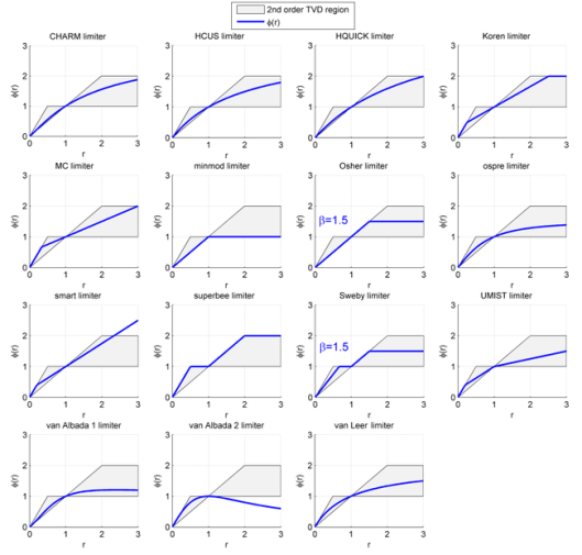A key part of the first generation’s methods success was the systematic justification for the form of limiters via a deep mathematical theory. This was introduced by Ami Harten with his total variation diminishing (TVD) methods. This nice structure for limiters and proofs of the non-oscillatory property really allowed these methods to take off. To amp things up even more, Sweby did some analysis and introduced a handy diagram to visualize the limiter and determine simply whether it fit the bill for being a monotone limiter. The theory builds upon some earlier work of Harten that showed how upwind methods provided a systematic basis for reliable computation through vanishing viscosity.

Simplicity is the ultimate sophistication.

― Clare Boothe Luce

The ground state method is upwind (donor cell) differencing, , which upon rearrangement shows that the new value, is a combination of positive definite values as long as . If the update to the new value is fully determined by positive coefficients, the result will be monotonicity preserving without any new extrema (new highs or lows not in the data). The TVD methods work in the same way except the coefficients for the update are now nonlinear and the conditions for the update being positive may produce conditions by which the update will be positive. I’ll focus on the simplest schemes possible using a forward Euler method in time, . For the upwind method this update is defined by using a positive direction for transport. For a generic second-order method one uses, where the use of linear extrapolation gives accuracy. Plugging this into the forward Euler update, and defining the extrapolation as a nonlinear function, . Now the update is written as, $ – 1/2 Q(j-1,n)) $ where . Now we can do some math using the assumption that does nothing to help matters insofar as keeping coefficients positive. We are left with a pretty simple condition for positivity as . If , the method is positive to ; if , $, the method is positive to . The point is that we now can concretely design schemes based on these inequalities that have reliable and well-defined properties.

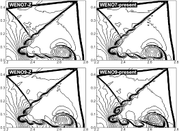The TVD and monotonicity-preserving methods while reliable and tunable through these functional relations have serious shortcomings. These methods have serious limitations in accuracy especially near detailed features in solutions. These detailed structures are significantly degraded because the methods based on these principles are only first-order accurate in these areas basically being upwind differencing. In mathematical terms this means that the solution are first-order in the L-infinity norm, approximately one-and-a-half in the L-2 (energy) norm and second-order in the L1 norm. The L1 norm is natural for shocks so it isn’t a complete disaster. While this class of method is vastly better than their linear predecessors effectively providing solutions completely impossible before, the methods are imperfect. The desire is to remove the accuracy limitations of these methods especially to avoid degradation of features in the solution.

The next generation of methods (the 2^nd nonlinear generation) sought to overcome these problems. The thing to avoid in the approximation is the utilization of first-order differencing at extreme values. While this is sensible, it is also dangerous. This is where new extrema in the solutions are created. This is where unphysical oscillations come from, and opens the door for all the things these methods are supposed to cure. The upshot of this is that getting rid of the detriments of the TVD methods requires being really careful. This care went into the creation of these methods, which were called essentially non-oscillatory methods (ENO). The gist of the design was to try and select the smoothest, smallest in magnitude variation differencing option locally.

Because of this the method tend to be very dissipative. This might seem odd at first glance, but consider that upwind differencing is based on a piecewise constant approximation within each cell. This is the lowest magnitude of variation possible, as such the small variation approximation within the cell used in ENO results in enhanced dissipation compared to TVD methods. This dissipative nature is one reason why these methods have not really been successful. The dissipative nature of ENO has recently been proven. It is a good thing in the sense that entropy satisfaction can be shown, but in some cases it can exceed that produced by upwinding. This is the second reason why ENO is not successful; exceeding upwind dissipation is actually a threat to stability of the scheme. Thus we have a method that is both low fidelity and lacking in robustness. This ends up being the price to pay for not degrading to a low order approximation at extrema and maintaining formal high-order accuracy there. Do we always have to pay this price? I don’t think so, and the median I talked about last week might allow us to get around the problem.

A big part of understanding the issues with ENO comes down to how the method works. The approximation is made through hierarchically selecting the smoothest approximation (in some sense) for each order and working ones way to high-order. In this way the selection of the second-order term is dependent on the first-order term, and the third-order term is dependent on the selected second-order term, the fourth-order term on the third-order one,… This makes the ENO method subject to small variations in the data, and prey to pathological data. For example the data could be chosen so that the linearly unstable stencil is preferentially chosen leading to nasty solutions. The safety of the relatively smooth and dissipative method makes up for these dangers. Still these problems resulted in the creation of the weighted ENO (WENO) methods that have basically replaced ENO for all intents and purposes.

WENO gets rid of the biggest issues with ENO by making the approximation much less sensitive to small variations in the data, and biasing the selection toward more numerically stable approximations. Moreover the solution to these issues allows for an even higher order approximation to be used if the solution is smooth enough to allow this. Part of the issue is the nature of ENO’s approach to approximation. ENO is focused on diminishing the dissipation at extrema, but systematically creates lower fidelity approximations everywhere else. If one looks at TVD approximations the “limiters” have a lot of room for non-oscillatory solutions if the solution is locally monotone. This is part of the power of these methods allowing great fidelity in regions away from extrema. By not capitalizing on this foundation, the ENO methods failed to build on the TVD foundation successfully. WENO methods come closer, but still produce far too much dissipation and too little fidelity to fully replace monotonicity-preservation in practical calculations. Nonetheless ENO and WENO methods are pragmatically and empirically known to be nonlinearly stable methods.

Given the lack of success of the second generation of methods, we have a great need for a third generation of nonlinear methods that might displace the TVD methods. Part of the issue with the ENO methods is the lack of a strict set of constraints to guide the development of the methods. While WENO methods also lack such constraints, they do have a framework that allows for design through the construction of the smoothness sensors, which help to determine the weights of the scheme. It allows for a lot of creativity, but the basic framework still leads to too much loss of fidelity compared to TVD methods. When one measures the accuracy of real solutions to practical problems WENO still has difficulty being competitive with TVD–don’t fooled by comparisons that show WENO being vastly better than TVD, the TVD method chosen to compare with is absolute shit. A good TVD method is very competitive, so the comparison is frankly disingenuous. For this reason something better is needed or progress will continue to stall.

My philosophy is to try and use the first two generations of nonlinear methods as the foundation. The median function is a means to allow the combining of the properties to get the best of both! This approach was taken in my 2007 paper with Jeff Greenough and Jim Kamm. As I stated then the objective is to get the best of both Worlds (TVD/monotonicity-preserving and ENO/WENO). Today I will explore if we can go even further.

The median comes in as a selection mechanism that allows beneficial properties to be built into methods. The three properties we will focus upon are listed here

• Numerical accuracy, both resolution/fidelity and order of accuracy
• Linear stability, or L2-energy stability
• Nonlinear stability, L1, variation or non-oscillatory

These properties if brought together in a provable manner should allow new methods to be crafted that may replace TVD methods in practical codes if all works together to produce accurate, high-fidelity, stable, non-oscillatory methods for producing better solutions efficiently.

The approach to take in producing better methods is to start as before with TVD methods, defining  where this edge value is defined as being high order accurate. If we can define inequalities that limit the values that may take we can have productive methods. This is very challenging because we cannot have purely positive definite coefficients if we want high-order accuracy, and we want to proceed forward beyond monotonicity-preservation. The issue that continues to withstand strict analysis is the determination of how large the negativity of coefficients may be and not create serious problems.

Satisfaction is the biggest hurdle to success

― Pushkar Saraf

The approach that I am advocating was described in last week’s post where the median function was used to “breed” new high-order approximations with appropriate linear and nonlinear stability properties. The “seed” for any given scheme will be a monotonicity-preserving–TVD method to act as the selector for the median. A good reason to use these methods is their nonlinear stability properties. Remember that the manner in which the median works requires at least two of the three arguments to have a property in order to assure that the evaluation of the function retains this property.

Dealing with this serious deficiency in a rigorous manner is extremely difficult. A philosophy to dealing with it may be to ignore the problem and introduce other mechanisms to make the solution robust. For example, use a positivity limiter approach to keep positive definite values, positive definite during the integration of the equation. These limiters are devilishly simple and drop into this numerical framework almost seamlessly. The limiter takes a minimum acceptable value and modifies the approximation to remove violations of that value in the evolution. The form is $ U(j+1/2,n) := U(j,n) + \theta\left( U(j+1/2,n) – U(j,n) \right) $ with $ \theta = \min \left( 1,\frac{ U_{\min} – U(j,n) }{ U(j+1/2,n) – U(j,n) } \right) $. The really awesome aspect of this limiter is its preservation of the accuracy of the original approximation. This could be extended to the enforcement of other bounds without difficulty.

The various extrema preserving limiters of Suresh and Huynh, Colella and Sekora or from myself along with Greenough and Kamm may be employed to good effect to keep the integration fully nonlinearly stable while allowing high-order accuracy. In every case these “limiters” or strategies are used to provide accurate approximations throughout the flow field being solved. It is opposed to the previous limiter where a non-local bound is enforced. By being more local the problem is more difficult and accuracy is more likely to be disturbed. The approaches taken before all work to detect extrema in the solutions and produce approximations that preserve extrema that are valid, but not produce new invalid extrema. A trap that this may fall into is only provide the capacity to produce solutions that are uniformly second-order accurate instead of the first-order accuracy that is standard with monotonicity-preservation. The problem with these approaches is their lack of rigorous and provable bounds or properties that helped drive the success of TVD methods. We will end by discussing an approach that might go to arbitrarily high-order without inducing extreme dissipation in the bulk of solution.

This approach is based on the properties of the median discussed last week. Given that we are going to gang up on bad approximations using the median by using two approximations with a desirable property to make sure any bad properties are removed. A really cool thing is getting rid of two bad approximations in one fell swoop. Take the following example, argument one is low-order, but linear and nonlinearly stable–upwind perhaps, or TVD, the second is linearly unstable (nonlinearly too), but high-order and the third is both high-order and nonlinearly stable. Using a median evaluation will produce a new approximation that is both nonlinear stable and high-order even if the evaluation does not return the original value with that property. This is a really powerful tool for getting what we are looking for!

More typically, we will focus on a single property in the evaluation of the median. In structuring and evaluating the tests one should carefully look at what common properties can be provably produced through any given test. The key is to use the evaluations to build up approximations with uniformly desirable properties. I gave several examples last week, and I will close with a new example that brings us closer to the goals set forth for a new generation of methods.

Let’s lay out the building blocks for our approximation scheme.

1. Have a TVD method, either a “classic” one, or a montonicity-preserving high-order scheme using the stencil described next.
2. Have an extra high-order method using a full stencil. This is analogous to the fifth-order WENO. Use a linear combination three third-order stencils to get a linear fifth-order scheme
3. One might also evaluate the fifth-order WENO method.
4. Finally have the three base third-order stencils recognizing that one of them is the “classic” ENO scheme.
5. Take inventory. You have three nonlinearly stable stencils, two fifth-order stencils, and three third-order stencils. You also have three or four linearly stable stencils.

Now let the median–magic happen right in front of you! Could one orchestrate the evaluations to give you a fifth-order, linearly and nonlinearly stable approximation? Can you really have it all? The answer, dear readers, is yes.

Here is how one might take on this challenge to systematically produce the desired result. Start with the playoff system discussed last week. This would use three median tests of the TVD scheme and the three third-order stencils. One of the third-order stencils is linearly unstable, and another is the classic ENO stencil, and is the third-order upstream-centered scheme – and upstream-centered is known to be very desirable. They might be the same one, or they might not, such is the nature of nonlinear stability. At the end of the three tests we now have a third-order scheme that is linearly and nonlinearly stable. Don’t take my word for it, lets take it all apart. The semi-finals would consist of two choices, and . Both and are third-order accurate and one of them is also nonlinearly stable to the extent that the ENO approximation would be, and another one is linearly stable in this case. Now we have the finals for step one, , this is nonlinearly stable and third-order, but linear stability isn’t necessarily given. For example the first-order method is linearly and nonlinear stable, or the second-order monotone Fromm’s scheme is linearly and nonlinearly stable. These two choices give the desired outcome guaranteed third-order, linear and nonlinearly stable schemes.

Now we can use a single additional test to promote things to a fifth-order version of the same. Our final test is . Here the third-order approximation has both desired stability properties, the fifth-order linear approximation–upsteam centered is linearly stable and the fifth-order WENO is nonlinear stable. The final evaluation has it all! Fifth-order! Linear stability! Nonlinear Stability! All using the magical mystical median!

Cherish those who seek the truth but beware of those who find it.

― Voltaire

There is still a lot to do. A few things stand out insofar as coming to more optimal methods. For example, is it a good idea to test the high-order approximation you’d like to use to see if it violates monotonicity, first? If it doesn’t, dispense with the whole survey of the other choices? What gives a better answer? In previous work this can yield big savings. In addition, the major issues with the monotone methods appear at extrema where almost all of the methods degrade to first-order accuracy. Getting safe, high fidelity approximations at extrema benefit from the sort of things done in the set of papers by myself and others trying to extend limiters. The extent to which new extrema would be created and manifesting themselves as some negative coefficients instead of positive definite monotonicity preserving approaches whose magnitude remain undefined by rigorous analysis. Similarly if the approximations are steeper than non-oscillation would allow in monotone regions of the flow, it would manifest itself as negative coefficients. The magnitude of the negativity and oscillation size is difficult to define. So far it does not appear to match the desired expectation of ENO schemes of being where is the order of the method, which might be as high as one likes. Evidence appears to go in the opposite direction insofar as WENO goes where the very high order WENO methods–higher than 7^th order appear to have larger oscillations and generic robustness issues.

What I will say is that the community of scientists building shock capturing methods do not as a rule measure the accuracy of the methods they work on under practical circumstances. Typically accuracy is only measured on problems where the design order of accuracy may be achieved. This characterizes none of the problems we develop such methods to solve! NONE! ZERO! NADA!

Thinking something does not make it true. Wanting something does not make it real.

― Michelle Hodkin

If we want continued improvement of methods we need to measure our progress! We need to get in the business of measuring the overall efficiency of the methods. The goal of producing a new generation of methods to replace the very successful first generation nonlinear methods should be focused on innovation with the purpose of producing better solutions for less effort along with deeply nonlinear stability, high-resolution and a reliable and robust framework allowing the method to adapt to the problem at hand. Today we avoid this like the proverbial plague and it serves no one, but a small cadre of insiders. It serves them poorly by maintaining an increasingly antiquated status quo, which only stands in the way of actual transformative progress.

While I’m dishing out dollops of cruel reality I should acknowledge that for practical problems there is a certain futility in seeking formally high-order accurate solutions. Almost everything necessary to model reality conspires against us. At every turn we are confronted with a brutal reality that offers us rough, and nearly singular behavior. To some extent the first generation methods reflect this brutish reality offering a pragmatic methodology. These methods simply reject any attempt at accuracy if the solution is too under-resolved or rough. Perhaps we must accept a degree of imperfection in the face of this truth?

There are two ways to get enough. One is to continue to accumulate more and more. The other is to desire less.

― G.K. Chesterton

The attempts to produce methods that robustly allow extrema in the solution to be evolved with less error effectively extend this principled submission to difficulty. They offer rather involved analysis of the extrema including explicit limits on their structure. The problem is that these methods have rather distinct limits on the accuracy that may be achieved with them. Maybe this is really OK? For too long we have pursued methods whose design and energy is driven by problems that are largely meaningless idealizations of the reality we should focus on. We might actually progress more effectively by accepting the intrinsic limitations of our models, and produce pragmatic improvements that manage the reality of their solution.

We all die. The goal isn’t to live forever, the goal is to create something that will.

― Chuck Palahniuk

References

Harten, Ami. “High resolution schemes for hyperbolic conservation laws.”Journal of computational physics 49.3 (1983): 357-393. Also. Harten, Ami. “High resolution schemes for hyperbolic conservation laws.”Journal of Computational Physics 135.2 (1997): 260-278. (see Harten, Ami. “On a class of high resolution total-variation-stable finite-difference schemes.” SIAM Journal on Numerical Analysis 21.1 (1984): 1-23. Too)

Sweby, Peter K. “High resolution schemes using flux limiters for hyperbolic conservation laws.” SIAM journal on numerical analysis 21.5 (1984): 995-1011.

Harten, Ami, Bjorn Engquist, Stanley Osher, and Sukumar R. Chakravarthy. “Uniformly high order accurate essentially non-oscillatory schemes, III.” Upwind and High-Resolution Schemes. Springer Berlin Heidelberg, 1987. 218-290. (see also Harten, Ami, Bjorn Engquist, Stanley Osher, and Sukumar R. Chakravarthy. “Uniformly high order accurate essentially non-oscillatory schemes, III.”Journal of Computational Physics 131, no. 1 (1997): 3-47.)

Harten, Ami, and Stanley Osher. “Uniformly high-order accurate nonoscillatory schemes. I.” SIAM Journal on Numerical Analysis 24.2 (1987): 279-309.

Fjordholm, Ulrik S., Siddhartha Mishra, and Eitan Tadmor. “Arbitrarily high-order accurate entropy stable essentially nonoscillatory schemes for systems of conservation laws.” SIAM Journal on Numerical Analysis 50.2 (2012): 544-573.

Fjordholm, Ulrik S., Siddhartha Mishra, and Eitan Tadmor. “ENO reconstruction and ENO interpolation are stable.” Foundations of Computational Mathematics 13.2 (2013): 139-159.

Jiang, Guang-Shan, and Chi-Wang Shu. “Efficient Implementation of Weighted ENO Schemes.” Journa of Computational Physics 126 (1996): 202-228.

Suresh, A., and H. T. Huynh. “Accurate monotonicity-preserving schemes with Runge–Kutta time stepping.” Journal of Computational Physics 136.1 (1997): 83-99.

Balsara, Dinshaw S., and Chi-Wang Shu. “Monotonicity preserving weighted essentially non-oscillatory schemes with increasingly high order of accuracy.”Journal of Computational Physics 160.2 (2000): 405-452.

Zhang, Xiangxiong, and Chi-Wang Shu. “Maximum-principle-satisfying and positivity-preserving high-order schemes for conservation laws: survey and new developments.” Proceedings of the Royal Society of London A: Mathematical, Physical and Engineering Sciences. Vol. 467. No. 2134. The Royal Society, 2011.

Rider, William J., Jeffrey A. Greenough, and James R. Kamm. “Accurate monotonicity-and extrema-preserving methods through adaptive nonlinear hybridizations.” Journal of Computational Physics 225.2 (2007): 1827-1848.

Colella, Phillip, and Michael D. Sekora. “A limiter for PPM that preserves accuracy at smooth extrema.” Journal of Computational Physics 227.15 (2008): 7069-7076. (see also Sekora, Michael, and Phillip Colella. “Extremum-preserving limiters for MUSCL and PPM.” arXiv preprint arXiv:0903.4200 (2009).)

 

Every solution to every problem is simple. It’s the distance between the two where the mystery lies.

― Derek Landy

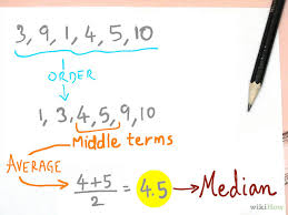The median is what a lot of people think of when you say “household income”. It is a statistical measure of central tendency of data that is a harder to compute alternative to the friendly common mean value. For large data sets the median is tedious and difficult to compute while the mean is straightforward and easy. The median is the middle entry of the ordered list of numerical data thus the data being studied needs to be ordered, which is hard and expensive to perform. The mean of the data is simple to compute. On the other hand by almost any rational measure, the median is better than the mean. For one thing, the median is not easily corrupted by any outliers in the data (data that is inconsistent or corrupted); it quite effectively ignores them. The same outliers immediately and completely corrupt the mean. The median is strongly associated with the one-norm, which is completely awesome and magical. This connection is explored through the amazing and useful field of compressed sensing, which uses the one norm to do some really sweet (cool, awesome, spectacular, …) stuff.

About 15 years ago I found myself quite taken with a mathematical tool associated with constructing “limiters” for solving hyperbolic conservation laws numerically. This mathematical tool is the “median” function for three arguments. It simply returns the value that lies in the middle of the triad. It simple and powerful, but hasn’t really caught on more generally. It seems to be a boutique method rather than common in use. It’s a true shame; because the median is pretty fucking awesome. Given the median’s power and utility in building numerical method, I find its lack of “popularity” puzzling. Since I like it so much, I will wax a bit on its greatness and what I’ve done with it.

It’s easy to attack and destroy an act of creation. It’s a lot more difficult to perform one.

― Chuck Palahniuk

I came across the function and its use with limiters reading the work of HT Huynh. HT works at NASA in Cleveland and has done some really great work over the years. The median function made its first appearance in work on Hermitian polynomial interpolation (used a lot with tabular lookups). He wrote several of my favorite papers on solving hyperbolic PDE’s, first on slope limited second-order schemes (a real gem covering a wealth of material and presenting it in a wonderful manner, it deserves many more citations!) and a second with Suresh on limiting edge values (another tour de force!). The median function appears prominently in both and allows some cool stuff to be done in a very clear and literal fashion. Like the median function, HT’s work is significantly under-appreciated.

If you want something new, you have to stop doing something old

― Peter F. Drucker

History is filled with brilliant people who wanted to fix things and just made them worse.

― Chuck Palahniuk

The function itself is quite elegant. If you’re in the business of limiters, you can implement it directly from another function you certainly have on hand, the minmod (minimum modulus) function. Jay Boris invented the minmod as part of the flux corrected transport method (arguably the first limiter). It returns the function with the minimum magnitude if the arguments to the function have the same sign, and zero otherwise. It can be implemented in several ways of varying elegance. The classic way of implementing minmod is, . HT Huynh introduced a really cool way to write minmod that was much better since you could use it with Taylor series expansions straightaway, .

Once the minmod is in hand, the median is a piece of cake to implement, . In papers by Huynh and Huynh & Suresh, the median is used to enforce bounds. This mindset is perfectly in keeping with the thinking about monotonicity preserving methods but the function has other properties that can take it much further. A lack of recognition of these other properties may limit its penetration into further use. In a general sense it is used in defining the limits that an approximation value can take and produce a monotonicity preserving answer. The median is used to repeatedly bring an approximate value inside well-defined bounding values although for monotonicity it just requires two applications. Huynh first applied this to the linear interpolated second-order methods. In that case the median could be used to implement the classical TVD limiters or slope limiters. Suresh and Huynh took the same approach to higher order accuracy through looking edge value/flux approximations that might have an arbitrary order of accuracy and integrated via a method of lines approach, but uses many other applications of the median in the process.

Do not get obsolete like an old technology, keep innovating yourself.

― Sukant Ratnakar

Once the median function is in hand it may be used to write limiters in what I think is a rather elegant fashion. For example take the standard monotonicity or TVD limiter for a “good” second-order method based on Fromm’s scheme, which can be written in a relatively hideous fashion as, . Here is the unlimited slope for the linear Fromm scheme, with – and  – being the negative and positive differences of the variables on the mesh. With the median we can write the limiter in two compact statements, , . More importantly as Huynh shows this format allows significant and profitable extensions of the approach leading to higher accuracy approximation. It is the extensibility that may be exploited as a platform to innovate limiters and remove some of their detrimental qualities.

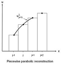The same basic recipe of bounding allows the parabolic limiter for the PPM method to be expressed quite concisely and clearly. The classic version of the PPM limiter involves “if” statements and seems rather unintuitive. With the median it is very clear and concise. The first simply assures that the chosen (high-order) edge values, and are enclosed by the neighboring mesh values, and . While the second step assures that the parabola does not contain a zero derivative (or no local minima or maxima) in the cell, – and – . With this version of PPM there is significant liberty in defining the left and right initial edge values by whatever formula, accuracy and nature you might like. This makes PPM an immensely flexible and powerful method (the original PPM is very powerful to begin with).

The median preserves accuracy and allows one to create new nonlinearly accurate approximations. Huynh delivered the median along with a theorem regarding it accuracy properties. If two of the three arguments in the median function have a certain order of accuracy in approximation than the evaluated median function will have that order of accuracy. The proof is simple and intuitive. If the defined order of accuracy values is returned there isn’t a question, but if the returned value does not have the order accuracy a priori, its accuracy is in question. By being bounded by the two values with well-defined linear order of accuracy, the median value is the convex combination of the two accurate values, which locally means it has the same order of accuracy. Viola! This means the median has the ability to “breed” new high order approximations from existing high-order expressions. If you’re interested in producing well-behaved approximations that are also high-order; it is a super useful property.

Here is a supposition that extends the accuracy property of the median to make it more powerful. The median can also “breed” new nonlinearly stable approximations. This would work as follows: if two of the arguments are stable, the evaluation of the median would produce a stable value even if the argument returned is linearly unstable. Thus we can take various stable approximations and through the median use them to produce new stable approximations even if they are unstable. This should work exactly like the order of approximation through the evaluated median producing a value that is the convex linear combination of the two defined stable approximations. If this property can be proven then all you need to do is keep track of the properties as you work defining your method. If you are careful you can end up with provable methods having well-defined accuracy and stability even when some parts of the method have neither to begin with. This is the essence of a the nonlinear method. It does something the linear method cannot.

This produced a concept of producing nonlinear schemes that I originally defined as a “playoff” system. The best accurate and stable approximation would be the champion of the playoffs and would inherit the properties of the set of schemes used to construct the playoff. This would work as long as the playoff was properly orchestrated to produce stable and high-order approximations in a careful manner if the median were used to settle the competition. I had discussed this as a way to produce better ENO-like schemes. Perhaps I should have taken the biological analogy in the definition of the scheme in terms of what sort of offspring each decision point in the scheme bred. Here the median is used to breed the schemes and produce more fit offspring. The goal at the end of scheme is to produce an approximation with a well-chosen order of accuracy and stability that can be proven.

The method I show here was developed with a goal in mind, produce an ENO(-like) method with all of the stability, but with better accuracy and fidelity. It would have the same order of accuracy as ENO methods, but would produce solutions of greater fidelity. One of the big issues with ENO (and WENO) methods is that they are relatively dissipative as well as being complex. For applied problems with shocks and discontinuous features a well-designed second-order method will produce a much better, higher fidelity solution than an ENO method. WENO is more competitive, but still not better than a method such as PPM until the solution has immense amount of high frequency structure. The goal is to produce ENO methods that inherit the sort of fidelity properties that second-order methods produce, but also provide bona fide high-order accuracy,

Here is a relatively simple example of the sort of scheme I suggested and how the “playoff” system would work. In this case, the goal is to produce a third-order approximation with well-defined stability properties. We start with three third order approximations, , and (all written from the right edge of cell ) plus a second-order monotone approximation . For example one might use the second-order minmod based scheme, . One of the three third-order methods is the upstream-centered scheme, which has favorable properties from an accuracy and stability point-of-view ( for this example).

The second thing to note is that one of the three third-order approximations is the nonlinearly stable classical ENO approximation (we don’t know which one, and don’t need to either! and that is cool). The playoff would consist of two rounds and three applications of the median in the process. The semi-finals would consist of two choices, and . Both and are third-order accurate and one of them is also nonlinearly stable to the extent that the ENO approximation would be (the second stable scheme is ). The finals then would be defined by the following test, and would produce a third-order and nonlinearly stable approximation. This is a direct consequence of the median function’s use. Two of the approximations are third-order, and two of the approximations are nonlinearly stable, so the result of the playoff final is an approximation that gives us both. The results from my paper strongly indicate that this approach is a success, and can be used to construct methods of much higher order accuracy.

If one were feeling more bold about solving problems of this ilk, one might throw the fifth-order upstream centered approximation into the mix. This fifth-order approximation is the asymptotic limit of the fifth-order WENO method when the solution is (very) smooth and a linear combination of the three third-order approximations, . Make the fifth-order approximation the returning champion have it play the winner of the playoff system in a final match. This would look like the following, . It would still only be third-order accurate in a formal manner, but have better accuracy where the solution is well-resolved. The other thing that is intrinsically different from the classic ENO approach is the guidance of the choice for . To a very large extent the result of the playoff is determined by this choice and the result inherits the properties of this method. There is a wealth of monotonicity-preserving second-order methods to choose from used to determine the fitness of the high-order approximations.

ENO methods traditionally use a hierarchical stencil selection approach that introduces serious practical problems. Their weighted version is a far better method (WENO) both because it is higher order, but also better stability properties. The high order nature of these schemes can be analyzed via the elegant continuous nature of the weights. The largest issue with both methods is their great cost either in floating point or logical expression evaluation. Using the median function can provide a route analogous to the playoff scheme above to produce an ENO method where the prospect is that the chosen scheme is the one closest to some “comparison” method chosen from the wealth of monotonicity-preserving methods. This ENO scheme would then inherit the basic properties of the base scheme, but also have the high-order nature of ENO along with being non-oscillatory. A close relative of the median function is the xmedian, which delivers whatever argument is closer in an absolute value sense to the comparison value. For the following form, the function will provide either or depending on their distance from . The function is written down at the end of the post along with all the other functions used (I came up with these to allow the analysis of this class of methods via modified equation analysis).

Here is a third-order ENO like method based on either the median or xmedian procedure. Both methods will produce a bona fide method with third-order accuracy (confirmed via numerical tests). The method starts with the selection of the comparison scheme, . This scheme may be first or second-order accurate, but needs to have strong nonlinear stability properties. For the third-order (or 4^th order) method, the scheme has two rounds and three total tests (i.e., semi-finals and finals). The semi-finals are and . The finals are then easy to predict from the previous method, $ latex U_{3,C} = \mbox{xmedian}\left( U_c, U_{3,A}, U_{3,B} \right) $. With the properties of the xmedian we can see that the scheme will select one of the third-order methods. This issue is that this playoff scheme does not produce a selection that would obviously be stable using the logic from earlier in the post. The question is whether the non-oscillatory method chosen by its relative closeness to the comparison scheme is itself nonlinearly stable.

The main question is the nature of the stability. The proposition is that the comparison scheme drawn from the category of nonlinear stable, monotonicity preserving methods endows the result with stability. With the median there is a very strong argument for stability. For the xmedian this argumentation is absent. Stability in both cases is born out through numerical testing, but theoretical support does not seem to have an obvious path. I note that ENO and WENO methods don’t have a deep stability result aside from the notion that classic ENO will produce an entropy-stable flux (but WENO does not). Practical success would seem to favor WENO to a very large degree as it has been applied to a vast number of practical cases.

If you’re not prepared to be wrong, you’ll never come up with anything original.

― Ken Robinson

The use of the median and related functions starts to beg some questions desperately in need of answers. There is a broad a deep of understanding of what numerical stability is and implies. This is for linear schemes, but the concept of nonlinear stability needs deeper thought. The archetypes of nonlinear stability are TVD/monotonicity-preserving schemes and ENO or WENO methods. The nature of these methods allows the local use of intrinsically unstable approximations without the usual path to catastrophe this implies. Where is the dividing line between a method being non-oscillatory (nonlinearly stable) and not. Using the median or its brother the xmedian, I can come up with a host of methods that perform in a fashion that implies that they are nonlinearly stable. Can we come up with a technically defensible definition that can be used to take these methods even further?

The possession of knowledge does not kill the sense of wonder and mystery. There is always more mystery.

― Anaïs Nin

References

Huynh, Hung T. “Accurate monotone cubic interpolation.” SIAM Journal on Numerical Analysis 30.1 (1993): 57-100.

Huynh, Hung T. “Accurate upwind methods for the Euler equations.” SIAM Journal on Numerical Analysis 32.5 (1995): 1565-1619.

Suresh, A., and H. T. Huynh. “Accurate monotonicity-preserving schemes with Runge–Kutta time stepping.” Journal of Computational Physics 136.1 (1997): 83-99.

Boris, Jay P., and David L. Book. “Flux-corrected transport. I. SHASTA, A fluid transport algorithm that works.” Journal of computational physics 11.1 (1973): 38-69. (Kuzmin, D., R. Löhner, and S. Turek, eds. Flux-Corrected Transport: Principles, Algorithms, and Applications. Scientific Computation. Springer, 2005.)

Balsara, Dinshaw S., and Chi-Wang Shu. “Monotonicity preserving weighted essentially non-oscillatory schemes with increasingly high order of accuracy.”Journal of Computational Physics 160.2 (2000): 405-452.

Colella, Phillip, and Paul R. Woodward. “The piecewise parabolic method (PPM) for gas-dynamical simulations.” Journal of computational physics 54.1 (1984): 174-201.

Rider, William J., Jeffrey A. Greenough, and James R. Kamm. “Accurate monotonicity-and extrema-preserving methods through adaptive nonlinear hybridizations.” Journal of Computational Physics 225.2 (2007): 1827-1848.

Harten, A., Engquist, B., Osher, S., & Chakravarthy, S. R. (1997). Uniformly high order accurate essentially non-oscillatory schemes, III. Journal of Computational Physics, 131(1), 3-47. (Harten, Ami, et al. “Uniformly high order accurate essentially non-oscillatory schemes, III.” Upwind and High-Resolution Schemes. Springer Berlin Heidelberg, 1987. 218-290.)

Liu, Xu-Dong, Stanley Osher, and Tony Chan. “Weighted essentially non-oscillatory schemes.” Journal of computational physics 115.1 (1994): 200-212.

Shu, Chi-Wang. Essentially non-oscillatory and weighted essentially non-oscillatory schemes for hyperbolic conservation laws. Springer Berlin Heidelberg, 1998.

Henrick, Andrew K., Tariq D. Aslam, and Joseph M. Powers. “Mapped weighted essentially non-oscillatory schemes: achieving optimal order near critical points.” Journal of Computational Physics 207.2 (2005): 542-567.

Greenough, J. A., and W. J. Rider. “A quantitative comparison of numerical methods for the compressible Euler equations: fifth-order WENO and piecewise-linear Godunov.” Journal of Computational Physics 196.1 (2004): 259-281.

Rider, William J. “Building Better (Weighted) ENO Methods.” Computational Fluid Dynamics 2006. Springer Berlin Heidelberg, 2009. 161-166.

Fjordholm, Ulrik S., Siddhartha Mishra, and Eitan Tadmor. “Arbitrarily high-order accurate entropy stable essentially nonoscillatory schemes for systems of conservation laws.” SIAM Journal on Numerical Analysis 50.2 (2012): 544-573.

Algebraically defined functions:

 

 

 

Clarke’s Third Law: Any sufficiently advanced technology is indistinguishable from magic.

– Arthur C. Clarke

One of the most important things about modern computational methods is their nonlinear approach to solving problems. These methods are easily far more important to the utility of modeling and simulation in the modern world than high performance computing. The sad thing is that little or no effort is going into extending and improving these approaches despite the evidence of their primacy. Our current investments in hardware are unlikely to yield much improvement whereas these methods were utterly revolutionary in their impact. The lack of perspective regarding this reality is leading to vast investment in computing technology that will provide minimal returns.

In this case the nonlinearity is the use of solution adaptive methods that apply the “best” method adjusted to the local structure of the solution itself. In many cases the methods are well grounded in theory, and provided the essential push of improvement in results that have powered computational physics into a powerful technology. Without these methods we would not have the capacity to reliably simulate many scientifically interesting and important problems, or utilize simulation in the conduct of engineering. The epitome of modeling and simulation success is computational fluid dynamics (CFD) where these nonlinear methods have provided the robust stability and stunning results capturing imaginations. In CFD these methods were utterly game changing and the success of the entire field is predicated on their power. The key to this power is poorly understood, and too often credited to computing hardware instead of the real source of progress: models, methods and algorithms with the use of nonlinear discretizations being primal. 

And a step backward, after making a wrong turn, is a step in the right direction.

― Kurt Vonnegut

Unfortunately, we live in an era where the power of these methods and algorithms is under-utilized. Instead we see an almost complete emphasis on computing hardware as the route toward progress. This emphasis is naïve, and ultimately limits the capacity of computing, modeling and simulation to become a boon to society. Our current efforts are utterly shallow intellectually and almost certainly bound to fail. This failure wouldn’t be the good kind of failure since the upcoming crash is absolutely predictable. Computing hardware is actually the least important and most distant aspect of computing technology necessary for the success of simulation. High performing computers are absolutely necessary, but woefully insufficient for success. A deeper and more appreciative understanding of nonlinear methods for solving our models would go a long way to harnessing the engine of progress.

When one thinks about these things that almost immediately comes to mind with nonlinear methods is the term “limiters”. Often limiters are viewed as being a rather heavy-handed and crude approach to things. A limiter is a term inherited from the physics community where physical effects in modeling and simulation need to be limited to stay within some prescribed physical bounds. For example keeping transport within the limit of the speed of light for radiation transport. Another example would be a limit keeping positive-definite quantities such as density or pressure, positive. In nonlinear methods the term limiter often can be interpreted as limiting the amount of high-order method used in solving an equation. It has been found that without limits high-order methods produce anomalous effects (e.g., oscillations, solutions outside bounds, non-positivity). The limiter becomes a mixing parameter for high-order and low-order method for solving a transport equation. Usually the proviso is that the low-order method is guaranteed to produce a physically admissible solution.

All theories are legitimate, no matter. What matters is what you do with them.

― Jorge Luis Borges

To keep from falling into the old traps of how to talk about things, let’s take a deeper look at how these things work, and why. Also explore the alternatives to limiters and the ways everything needs to work together to be effective. There is more than one way to make it all work, but the recipe ends up being quite the same at the high end.

Ideally, we would like to have highly accurate, very stable, and completely reliable computations. The fundamental nature of our models of the universe conspire to make this far from a trivial task. Our models being comprised of mathematical expressions then are governed by mathematical realities. These realities in the form of fundamental theorems provide a foundation upon which excellent numerical methods may be built. Last week I discussed the Lax Equivalence theorem and this is a good place to start. There the combination of consistency and stability imply convergence of solutions. Consistency is having numerical accuracy if at least first order, but higher than first order accuracy will be more efficient. Stability is the nature of just getting a solution that hangs together (doesn’t blow up as we compute it). Stability is something so essential to success that it supersedes anything else when it is absent. Next in our tour of basic foundational theorems is Godunov’s theorem, which tells us a lot about what is needed. In its original form it’s a bit of a downer, you can’t have a linear method be higher than first-order accurate and non-oscillatory (monotonicity preserving). The key concept is to turn the barrier on its head, you can have a nonlinear method be higher than first-order accurate and non-oscillatory. This is then the instigation for the topic of this post, the need and power of nonlinear methods. I’ll posit the idea that the concept may actually go beyond hyperbolic equations, but the whole concept of nonlinear discretizations is primarily applied to hyperbolic equations.

A few more theorems help to flesh out the basic principles we bring to bear. A key result is the theorem of Lax and Wendroff that shows the value of discrete conservation. If one has conservation then you can show that you are achieving weak solutions. This must be combined with picking the right weak solution, as there are actually infinitely many weak solutions, all of them wrong save one. The task of getting the right weak solution is produced with sufficient dissipation, which produces entropy. Key results are due to Osher who attached the character of (approximate) Riemann solvers to the production of sufficient dissipation to insure physically relevant solutions. As we will describe there are other means to introducing dissipation aside from Riemann solvers, but these lack some degree of theoretical support unless we can tie them directly to the Riemann problem. Of course most of us want physically relevant solutions although lots of mathematicians act like this is not a primal concern! There is a vast phalanx of other theorems of practical interest, but I will end this survey with a last one by Osher and Majda with lots of practical import. Simply stated this theorem limits the numerical accuracy we can achieve in regions affected by a discontinuous solution to first-order accuracy. The impacted region is bounded by the characteristics emanating from the discontinuity. This puts a damper on the zeal for formally high order accurate methods, which needs to be considered in the context of this theorem.

Whenever a theory appears to you as the only possible one, take this as a sign that you have neither understood the theory nor the problem which it was intended to solve.

― Karl Popper

I will note that we are focused on hyperbolic equations because they are so much harder to solve. It remains an open question as to how much all of this applies to parabolic or elliptic equations. I suspect it does albeit to a less degree because those equations are so much more forgiving. Hyperbolic equations are deeply unforgiving and cause you to pay for all sins many times over. For this reason hyperbolic equations have been a pacing aspect of computational modeling where nonlinear methods have allowed progress and to some degree tamed the demons.

Let’s return to the idea of limiters and act to dissuade the common view of limiters and their intrinsic connection to dissipation. The connection there is real, but less direct than commonly acknowledged. A limiter is really a means of stencil selection in an adaptive manner separate from dissipation. They may be combined, but usually not with good comprehension of the consequences. Another way to view the limiter is a way of selecting the appropriate bias in the stencil used to difference an equation based upon the application of a principle. The principle most often used for limiting is some sort of boundedness in the representation, which may equivalently be associated with selecting a smoother (nicer) neighborhood to execute the discretization on. The way an equation is differenced certainly impacts the nature and need for dissipation in the solution, but it is indirect. Put differently, the amount of dissipation needed with the application of a limiter varies both with the limiter itself, but also with the dissipation mechanism, but the two are independent. This does get into the whole difference between flux limiters and geometric limiters, a topic worth some digestion.

In examining the topic of limiters and nonlinear stabilization we find an immediate and significant line of demarcation between two philosophical tenets. The first limiters came from limiting fluxes in the method of flux corrected transport. An alternative approach is found through extending Godunov’s method to higher order accuracy, and involves the limiting of the geometric reconstruction of variables. In the case of flux limiting, the accuracy and dissipation (e.g. stabilization) are mixed together while the geometric approach separates these effects into independent steps. The geometric approach puts bounds on the variables being solved, and then relies on an agnostic approach to the variables for stabilization in the form of a Riemann solver. Both approaches are successful in solving complex systems of equations and have their rabid adherents (I favor the reconstruct-Riemann approach). The flux form can be quite effective and produces better extensions to multiple dimensions, but can also involve heavy-handed dissipation mechanisms.

If one follows the path using geometric reconstruction several aspects of nonlinear stabilization may be examined more effectively. Many of the key issues associated with the nonlinear stabilization are crystal clear in this context. The clearest example is monotonicity of the reconstruction. It is easy to see how the reconstructed version of the solution is bounded (or not) compared to the local variable’s bounds. It is generally appreciated that the application of monotonicity renders solutions relatively low order in accuracy. This is most acute at extrema in the solution where the accuracy degrades to first-order intrinsically. What becomes even more enabled by looking at the geometric reconstruction is moving beyond monotonicity to stabilization that provides better accuracy. The derivation of methods that do not degrade accuracy at extrema, but extend the concept of boundedness appropriately is much clearer with a geometric approach. Solving this problem effectively is a key to producing methods with greater numerical accuracy and better efficiency computationally. While this may be achieved via flux limiters with some success there are serious issues in conflating geometric fidelity with dissipative stabilization mechanisms.

The needs for dissipation in schemes are often viewed with significant despair by parts of the physics community. Much of the conventional wisdom would dictate that dissipation-free solutions are favored. This is rather unfortunate because dissipation is the encoding of powerful physics principles into methods rather than some sort of crude numerical artifice. Their specific and bounded dissipative character governs most complex nonlinear systems. If the solution has too little dissipation, the solution is not physical. As such, dissipation is necessary and its removal could be catastrophic.

The first stabilization of numerical methods was found with the original artificial viscosity (developed by Robert Richtmyer to stabilize and make useful John Von Neumann’s numerical method for shock waves). The name “artificial viscosity” is vastly unfortunate because the dissipation is utterly physical. Without its presence the basic numerical method was utterly and completely useless leading to a catastrophic instability (almost certainly helped instigate the investigation of numerical stability along with instability in integrating parabolic equations). Physically most interesting nonlinear systems produce dissipation even in the limit where the explicit dissipation can be regarded as vanishingly small. This is true for shock waves and turbulence where the dissipation in the inviscid limit hasremarkably similar forms structurally. Given this basic need, the application of some sort of stabilization is an absolute necessity to produce meaningful results both from a purely numerical respect and the implicit connection to the physical World. I’ve written recently on the use of hyperviscosity as yet another mechanism for producing dissipation. Here the artificial viscosity is the archetype of hyperviscosity and its simplest form. As I’ve mentioned before the original turbulent subgrid model was also based directly upon the artificial viscosity devised by Richtmyer (often misattributed to Von Neumann although their collaboration clearly was important).

The other approach to stabilization is at first blush utterly different in approach, but upon deep reflection completely similar and complementary. For other numerical methods the use of Riemann solvers can be used to provide stability. A Riemann solver uses the nature of a local (approximate) exact physical solution to resolve a flow locally. In this way the nature of the physical propagation of information provides a more stable representation of the solution. It turns out that the Riemann solution will produce an implicit dissipative effect that impacts the solution much like artificial viscosity would. The real power is exploiting this implicit dissipative effect to provide real synergy where each may provide complementary views of stabilization. For example a Riemann solver produces a complete image of what modes in a solution must be stabilized in a manner that might inform the construction of an improved artificial viscosity. On the other hand artificial viscosity applies to nonlinearities often ignored by approximate Riemann solvers. Finding an equivalence between the two can produce more robust and complete Riemann solvers. As is true with most things, true innovation can be achieved through an openmind and a two way street.

Perhaps I will attend to a deeper discussion of how high-order accuracy connects to these ideas in next week’s post. I’ll close with a bit of speculation. In my view one of the keys to the future is how to figure out how to efficiently harness high-order methods for more accurate solutions with sufficient robustness. New computing platforms dearly need the computational intensity offered by high-order methods to keep themselves busy in auseful manner because of exorbitant memory access costs. Because practical problems are ugly with all sorts of horrible nonlinearities and effectively singular features, the actual attainment of high-order convergence of solutions is unachievable. Making high-order methods both robust enough and efficient enough under these conditions has thus far eluded our existing practice.

Extending the ideas of nonlinear methods to other physics is another direction needed. For example, do any of these ideas apply to parabolic equations with high-order methods? There are some key ideas of physically relevant solutions, but parabolic equations are generally so forgiving no focus is given. The question of whether something like Godunov’s theorem applying to high-order solution of parabolic equations is worth asking (I think a modified version of it might well). I will not that some non-oscillatory schemes do apply to extremely nonlinear parabolic equations exhibiting wave-like solutions.

The last bit of speculation will apply to the application of these ideas to common methods for solid mechanics. Generally it has been found that artificial viscosity is needed for stabling integrating solid mechanical models. Unfortunately this is using the crudest and least justified philosophy of artificial viscosity. Solid mechanics could deeply utilize the principles of nonlinear methods to very great effect. Solid mechanics is basically a system hyperbolic equations abiding by the full set of foundational conditions elucidated earlier in the post. As such everything should follow as a matter of course. Today this is not the case and my belief is that the codes suffer greatly from a lack of robustness and deeper mathematical foundation for the modeling and simulation capability.

The success of modeling and simulation as a technological tool and engine of progress would be well served by focus on nonlinear discretization lacking almost entirely from our current emphasis on hardware.

The reasonable man adapts himself to the world: the unreasonable one persists in trying to adapt the world to himself. Therefore all progress depends on the unreasonable man.

― George Bernard Shaw

References

VonNeumann, John, and Robert D. Richtmyer. “A method for the numerical calculation of hydrodynamic shocks.” Journal of applied physics 21.3 (1950): 232-237.

Lax, Peter D., and Robert D. Richtmyer. “Survey of the stability of linear finite difference equations.” Communications on Pure and Applied Mathematics 9.2 (1956): 267-293.

Godunov, Sergei Konstantinovich. “A difference method for numerical calculation of discontinuous solutions of the equations of hydrodynamics.”Matematicheskii Sbornik 89.3 (1959): 271-306.

Lax, Peter, and Burton Wendroff. “Systems of conservation laws.”Communications on Pure and Applied mathematics 13.2 (1960): 217-237.

Osher, Stanley. “Riemann solvers, the entropy condition, and difference.”SIAM Journal on Numerical Analysis 21.2 (1984): 217-235.

Majda, Andrew, and Stanley Osher. “Propagation of error into regions of smoothness for accurate difference approximations to hyperbolic equations.”Communications on Pure and Applied Mathematics 30.6 (1977): 671-705.

Harten, Amiram, James M. Hyman, Peter D. Lax, and Barbara Keyfitz. “On finite‐difference approximations and entropy conditions for shocks.”Communications on pure and applied mathematics 29, no. 3 (1976): 297-322.

Boris, Jay P., and David L. Book. “Flux-corrected transport. I. SHASTA, A fluid transport algorithm that works.” Journal of computational physics 11.1 (1973): 38-69.

Zalesak, Steven T. “Fully multidimensional flux-corrected transport algorithms for fluids.” Journal of computational physics 31.3 (1979): 335-362.

Van Leer, Bram. “Towards the ultimate conservative difference scheme. V. A second-order sequel to Godunov’s method.” Journal of computational Physics 32.1 (1979): 101-136.

Van Leer, Bram. “Towards the ultimate conservative difference scheme. IV. A new approach to numerical convection.” Journal of computational physics23.3 (1977): 276-299.

Liu, Yuanyuan, Chi-Wang Shu, and Mengping Zhang. “High order finite difference WENO schemes for nonlinear degenerate parabolic equations.”SIAM Journal on Scientific Computing 33.2 (2011): 939-965.

 

 

Not trying or putting forth your best effort is.

Only those who dare to fail greatly can ever achieve greatly.

― Robert F. Kennedy

Last week I attended the ASME Verification and Validation Symposium as I have for the last five years. One of the keynote talks ended with a discussion of the context of results in V&V. It used the following labels for an axis: Success (good) and Failure (bad). I took issue with it, and made a fairly controversial statement. Failure is not negative or bad, and we should not keep referring to it as being negative. I might even go so far as to suggest that we actually encourage failure, or at the very least celebrate it because failure also implies your trying. I would be much happier if the scale was related to effort and excellence of work. The greatest sin is not failing; it is not trying.

Keep trying; success is hard won through much failure.

― Ken Poirot

It is actually worse than simply being a problem that the best effort isn’t put forth, lack of acceptance of failure inhibits success. The outright acceptance of failure as a viable outcome of work is necessary for the sort of success one can have pride in. If nothing is risked enough to potentially fail than nothing can be achieved. Today we have accepted the absence of failure as being the tell tale sign of success. It is not. This connection is desperately unhealthy and leads to a diminishing return on effort. Potential failure while an unpleasant prospect is absolutely necessary for achievement. As such the failures when best effort is put forth should be celebrated and lauded whenever possible and encouraged. Instead we have a culture that crucifies those who fail with regard for the effort on excellence of the work going into it.

Right now we are suffering in many endeavors from deep unremitting fear of failure. The outright fear of failing and the consequences of that failure are resulting in many efforts reducing their aggressiveness in attacking their goals. We reset our goals downward to avoid any possibility of being regarded as failing. The result is an extensive reduction in achievement. We achieve less because we are so afraid of failing at anything. This is resulting is the destruction of careers, and the squandering of vast sums of money. We are committing to mediocre work that is guaranteed of “success” rather than attempting excellent work that could fail.

A person who never made a mistake, never tried anything new

― Albert Einstein

We have not recognized the extent to which failure energizes our ability to learn, and bootstrap ourselves to a greater level of achievement. Failure is perhaps the greatest means to teach us powerful lessons. Failure is a means to define our limits of understanding and knowledge. Failure is the fuel for discovery. Where we fail, we have work that needs to be done. We have mystery and challenge. Without failure we lose discovery, mystery, challenge and understanding. Our knowledge becomes stagnant and we cease learning. We should be embracing failure because failure leads to growth and achievement.

Instead today we recoil and run from failure. Failure has become such a massive black mark professionally that people simply will not associate themselves with something that isn’t a sure thing. The problem is that sure things aren’t research they are developed science and technology. If one is engaged in research, we do not have certain results. The promise of discovery is also tinged with the possibility of failure. Without the possibility of failure, discovery is not possible. Without an outright tolerance for a failed result or idea, the discovery of something new and wonderful cannot be had. At a personal level the ability to learn, develop and master knowledge is driven by failure. The greatest and most compelling lessons in life are all driven by failures. With a failure you learn a lesson that sticks with you, and your learning sticks.

Creatives fail and the really good ones fail often.

― Steven Kotler

It is the ability to tolerate ambiguity in results that leads to much of the management response. Management is based on assuring results and defining success. Our modern management culture seems to be incapable of tolerating the prospect of failure. Of course the differences in failure are not readily supported by our systems today. There is a difference between an earnest effort that still fails and an incompetent effort that fails. One should be supported and celebrated and the other is the definition of unsuccessful. We have lost the capacity to tolerate these subtleties. All failure is viewed as the same and management is intolerant. They require results that can be predicted and failure undermines this central tenant of management.

The end result of all of this failure avoidance is a generically misplaced sense of what constitutes achievement. More deeply we are losing the capacity to fully understand how to structure work so that things of consequence may be achieved. In the process we are wasting money, careers and lives in the pursuit of hollowed out victories. The lack of failure is now celebrated even though the level of success and achievement is a mere shadow of the sorts of success we saw a mere generation ago. We have become so completely under the spell of avoidance of scandal that we shy away from doing anything bold or visionary.

We live in an age where the system cannot tolerate a single bad event (e.g., failure whether it is an engineered system, or a security system,…). In the real World failures are utterly and completely unavoidable. There is a price to be paid for reductions of bad events and one can never have an absolute guarantee. The cost of reducing the probability of bad events escalates rather dramatically as you look to reduce the tail probabilities beyond a certain point. Things like the mass media and demagoguery by politicians takes any bad event and stokes fears using the public’s response as a tool for their own power and purposes. We are shamelessly manipulated to be terrified of things that have always been one-off minor risks to our lives. Our legal system does its dead level best to amp all of this fearful behavior for their own selfish interests of siphoning as much money as possible from whoever has the misfortune of tapping into the tails of extreme events.

In the area of security, the lack of tolerance for bad events is immense. More than this, the pervasive security apparatus produces a side effect that greatly empowers things like terrorism. Terror’s greatest weapon is not high explosives, but fear and we go out of our way to do terrorists jobs for them. Instead of tamping down fears our government and politicians go out of their way to scare the shit out of the public. This allows them to gain power and fund more activities to answer the security concerns of the scared shitless public. The best way to get rid of terror is to stop getting scared. The greatest weapon against terror is bravery, not bombs. A fearless public cannot be terrorized.

The end result of all of this risk intolerance is a lack of achievement as individuals, organizations, or the society itself. Without the acceptance of failure, we relegate ourselves to a complete lack of achievement. Without the ability to risk greatly we lack the ability to achieve greatly. Risk, danger and failure all improve our lives in every respect. The dial is too turned away from accepting risk to allow us to be part of progress. All of us will live poorer lives with less knowledge, achievement and experience because of the attitudes that exist today. The deeper issue is that the lack of appetite for obvious risks and failure actually kicks the door open for even greater risks and more massive failures in the long run. These sorts of outcomes may already be upon us in terms of massive opportunity cost. Terrorism is something that has cost our society vast sums of money and undermined the full breadth of society. We should have had astronauts on Mars already, yet the reality of this is decades away, so our societal achievement is actually deeply pathetic. The gap between “what could be” and “what is” has grown into a yawning chasm. Somebody needs to lead with bravery and pragmatically take the leap over the edge to fill it.

We have nothing to fear but fear itself.

– Franklin D. Roosevelt.

 

Advances are made by answering questions. Discoveries are made by questioning answers. Bernard Haisch

― Philip Houston

In the constellation of numerical analysis theorems the Lax equivalence theorem may have no equals in its importance. It is simple and its impact is profound on the whole business of numerical approximations. The theorem basically implies that if you provide a consistent approximation to the differential equations of interest and it is stable, the solution will converge. The devil of course is in the details. Consistency is defined by having an approximation with ordered errors in the mesh or time discretization, which implies that the approximation is at least first-order accurate, if not better. A key aspect of this that is overlooked is the necessity to have mesh spacing sufficiently small to achieve the defined error where failure to do so renders the solution erratically convergent at best.

The importance of this theorem in the basis for our commitment to high performance computing cannot be understated. The generally implicit assumption that more computer power is the path to better calculation is incredibly widespread. The truth and limits of this assumption are important to understand. If things are working well, it is a good assumption, but it should not be taken for granted. A finer mesh is almost a priori assumed to be better. This basic premise is rarely if ever challenged, but it should be. Under ideal circumstances it is a fine assumption, but it is not challenged nearly as often as it should be. Part of this narrative is the description of when it should be challenged and the nature of circumstances where verification achieves outright conflict with the utility of the model. We end with the prospect that the verified model might only be accurate and verified in cases where the model is actually invalid.

For example we can carry out a purely mathematical investigation of the convergence of a numerical solution without any regard for its connection to a models utility. Thus we can solve a problem using time and length scales that would render the underlying model as ridiculous and satisfy the mathematical conditions we are examining. Stepping away from this limited perspective to look at the combination of convergence with model utility is necessary. In practical terms the numerical error and convergence where a model is valid is essentially important to understand. Ultimately we need accurate numerical solutions in regimes where a model is valid. More than just being accurate, we need to understand what the numerical errors are in these same regions. Too often we see meshes refined to a ridiculous degree without regard to whether the length scales in the mesh render the model invalid.

I have always thought the actions of men the best interpreters of their thoughts.

― John Locke

A second widespread and equally troubling perspective is the wrong-headed application of the concept of grid independent solutions. Achieving a grid-independent solution is generally viewed as a good to great thing. It is if the conditions are proper. It is not under almost identical conditions. The difference between the good almost great thing, and the awful almost horrible thing is a literal devil in the details, but essential to the conduct of excellence in computational science. One absolutely must engage in the quantitative interrogation of the results. Without a quantitative investigation, the good grid independent results could actually be an illusion.

If the calculation is convergent, the grid independence actually means the calculation is not sensitive to the grid in a substantive manner. This requires that the solution have small errors and the grid independence is the effect of those errors being ordered and negligible. In fact it probably means that you’re engaged in overkill and could get away with a coarser (cheaper) grid without creating any substantial side effects. On the other hand a grid independent solution could mean that the calculation is complete garbage numerically because the grid doesn’t affect the solution. It is not convergent. These two cases are virtually identical in practice and only revealed by doing detailed quantitative analysis of the results. In the end grid independence isn’t either necessary, or sufficient for quality computations. Yet at the same time it is often the advised course of action in conducting computations!

Stability then becomes the issue where you must assure that the approximations produce bounded results under the appropriate control of the solution. Usually the stability is defined as a character of the time stepping approach and requires that the time step be sufficiently small to provide stability. A lesser-known equivalence theorem is due to Dahlquist and applies to integrating ordinary differential equations and applies to multistep methods. From this work the whole aspect of zero stability arises where you have to assure that a non-zero time step size gives stability in the first place. More deeply, Dahlquist’s version of the equivalence theorem applies to nonlinear equations, but is limited to multistep methods where as Lax’s applies to linear equations.

Here is the theorem in all its glory (based on wikipedia entries).

The Lax Equivalence Theorem:

For the numerical solution of partial differential equations. It states that for a consistent finite difference method for a well-posed linear initial value problem, the method is convergent if and only if it is stable. Published in 1956, discussed in a seminar by Lax in 1954.

The Dahlquist Equivalence Theorem:

Now suppose that a consistent linear multistep method is applied to a sufficiently smooth differential equation and that the starting values  all converge to the initial value  as . Then, the numerical solution converges to the exact solution as  if and only if the method is zero-stable.

Something to take serious note of regarding these theorems is the concept of numerical stability was relatively new and novel in 1956. Both theorems helped to lock the concept of stability into being central to numerical analysis. As such both theorems have place as one of the cornerstones of modern numerical analysis. The discovery of the issue of stability was first addressed by Von Neumann for PDEs in the late 1940’s, and independently explored by Dahlquist for ODEs in the early 1950’s. Nonetheless it should be noted that these theorems were published when numerical stability was a new concept and not completely accepted and understood for its importance.

Given that we can very effectively solve nonlinear equations using the principles applied by Lax’s theorem is remarkable. Even though the theorem doesn’t formally apply to the nonlinear case the guidance is remarkably powerful and appropriate. We have a simple and limited theorem that produces incredible consequences for any approximation methodology that we are applying to partial differential equations. Moreover the whole this was derived in the early 1950’s and generally thought through even earlier. The theorem came to pass because we knew that approximations to PDEs and their solution on computers do work. Dahlquist’s work is founded on a similar path; the availability of the computers shows us what the possibilities are and the issues that must be elucidated. We do see a virtuous cycle where the availability of computing capability spurs on developments in theory. This is an important aspect of healthy science where different aspects of a given field push and pull each other. Today we are counting on hardware advances to push the field forward. We should be careful that our focus is set where advances are ripe, its my opinion that hardware isn’t it.

The equivalence theorem also figures prominently in the exercise of assuring solution quality through verification. This requires the theorem to be turned ever so slightly on its head in conducting the work. Consistency is not something that can be easily demonstrated; instead verification focuses on convergence, which may be. We can control the discretization parameters, mesh spacing or time step size to show how the solution changes with respect to them. Thus in verification, we use the apparent convergence of solutions to imply both stability and consistency. Stability is demonstrated by fiat in that we have a bounded solution to use to demonstrate convergence. Having a convergent solution with ordered errors then provides consistency. The whole thing barely hangs together, but makes for the essential practice in numerical analysis.

At this time we are starting to get at the practical limitations of this essential theorem. One way to get around the issues is the practice of hard-nosed code verification as a tool. With code verification you can establish that the code-discretization produces the correct solution to an exact solution to the PDEs. In this way the consistency of the approximation can become firmly established. Part of the remaining issue is the fact that the analytical exact solution is generally far nicer and better behaved that the general solutions you will be applying the code to. Still this is a vital and important step in the overall practice. Without firm code verification as a foundation, the practice of verification without exact solutions is simply untethered. Here we have firmly established the second major limitation of the equivalence theorem, the first being it’s being limited to linear equations.
One of the very large topics in V&V that is generally overlooked is models and their range of validity. All models are limited in terms of their range of applicability based on time and length scales. For some phenomena this is relatively obvious, e.g., multiphase flow. For other phenomena the range of applicability is much more subtle. Among the first important topics to examine is the satisfaction of the continuum hypothesis, the capacity of a homogenization or averaging to be representative. The degree of satisfaction of homogenization is dependent on the scale of the problem and degrades as phenomenon becomes smaller scale. For multiphase flow this is obvious as the example of bubbly flow shows. As the number of bubbles becomes smaller any averaging becomes highly problematic. It argues that the models should be modified in some fashion to account for the change in scale size.

I’ll get at another extreme example of the nature of scale size and the capacity of standard models to apply. Take the rather pervasive principle associated with the second law of thermodynamics. As the size of the system being averaged becomes smaller and smaller eventually violations of this law can be occasionally observed. This clearly means that natural and observable fluctuations may cause the macroscopic laws to be violated. The usual averaged continuum equations do not support this behavior. It would imply that the models should be modified for appropriate scale dependence where such violations in the fundamental laws might naturally appear in solutions.

Another more pernicious and difficult issues are homogenization assumptions that are not so fundamental. Consider the situation where a solid is being modeled in a continuum fashion. When the mesh is very large, the solid comprised of discrete grains can be modeled by averaging over these grains because there are so many of them. Over time we are able to solve problems with smaller and smaller mesh scales. Ultimately we now solve problems where the mesh size approaches the grain size. Clearly under this circumstance the homogenization used for averaging will lose its validity. The structural variations in the homogenized equations are removed and should become substantial and not be ignored as the mesh size becomes small. In the quest for exascale computing this issue is completely and utterly ignored. Some areas of study for high performance computing consider these issues carefully most notably climate and weather modeling where the mesh size issues are rather glaring. I would note that these fields are subjected to continual and rather public validation.

Let’s get to some other deeper limitations of the power of this theorem. For example the theorem gets applied to the models without any sense of the validity of the model. Without consideration for validity, the numerical exploration of convergence may be explored with vigor and be utterly meaningless. The notion of validation is important in considering whether verification should be explored in depth. As such one gets to the nature of V&V as holistic and iterative. As such the overall exploration should always look back at results to determine whether everything is consistent and complete. If the verification exercise takes the model outside its region of validity, the verification error estimation may be regarded as suspect.

The theorem is applied to the convergence of the model’s solution in the limit where the “mesh” spacing goes to zero. Models are always limited in their applicability as a function of length and time scale. The equivalence theorem will be applied and take many models outside their true applicability. An important thing to wrangle in the grand scheme of things is whether models are being solved and convergent in the actual range of scales where it is applicable. A true tragedy would be a model that is only accurate and convergent in regimes where it is not applicable. This may actually be the case in many cases most notably the aforementioned multiphase flow. This calls into question the nature of the modeling and numerical methods used to solve the equations.

Huge volumes of data may be compelling at first glance, but without an interpretive structure they are meaningless.

― Tom Boellstorff

The truth is we have an unhealthy addiction to high performance computing as a safe and trivial way to make progress computationally. We continually move forward with complete faith that a larger calculations are intrinsically better without doing the legwork to demonstrate that they are. We avoid focus on other routes to better solutions in modeling, methods and algorithms in favor of simply porting old models, methods and algorithms to much larger computers. Without having a balanced program with appropriate intellectual investment and ownership of the full breadth of computational science, our approach is headed for disaster. We have a significant risk of producing a computational science program that completely fools itself. We fail to do due diligence activities in favor of simply making the assumption that a finer mesh computed on bigger computers is a priori better than taking another route to improvement.

The difficulty lies not so much in developing new ideas as in escaping from old ones.

― John Maynard Keynes

Lax, Peter D., and Robert D. Richtmyer. “Survey of the stability of linear finite difference equations.” Communications on Pure and Applied Mathematics 9.2 (1956): 267-293.

 

Dahlquist, Germund. “Convergence and stability in the numerical integration of ordinary differential equations.” Mathematica Scandinavica 4 (1956): 33-53.

 

…fuck?

WTF has become the catchphrase for today’s world. “What the fuck” moments fill our days and nothing is more WTF than Donald Trump. We will be examining the viability of the reality show star, and general douchebag celebrity-rich guy as a viable presidential candidate for decades to come. Some view his success as a candidate apocalyptically, or characterize it as an “extinction level event” politically. In the current light it would seem to be a stunning indictment of our modern society. How could this happen? How could we have come to this moment as a nation where it is even a possibility for such a completely insane outcome to be a reasonably high probability outcome of our political process? What else does it say about us as a people? WTF? What in the actual fuck!

The phrase “what the fuck” came into the popular lexicon along with Tom Cruz in the movie, “Risky Business” back in 1983. There the lead character played by Tom Cruz exclaims, “sometimes you gotta say, what the fuck” It was a mantra for just going for broke and trying stuff without obvious regard for the consequences. Given our general lack of an appetite for risk and failure, the other side of the coin took the phrase over. Over time the phrase has morphed into a general commentary about things that are generally unbelievable. Accordingly the acronym WTF came into being by 1985. I hope that 2016 is peak-what the fuck, cause things can’t get much more what the fuck without everything turning into a complete shitshow. Going to a deeper view of things the real story behind where we are is the victory of bullshit as a narrative element in society. In a sense the transfer of WTF from a mantra for risk taking has transmogrified into a mantra for the breadth of impact of not taking risks!

Indeed if one looks to the real core of the Donald Trump phenomena it is the victory of bullshit over logic, facts and rational thought. He simply spouts off a bunch of stuff that our generally uneducated, bigoted, and irrationally biased public wants to hear, and the rubes vote for him in droves. It does not matter that almost everything he says is complete and utter bullshit. A deeper question is how the populace has become so conditioned to accept a candidate who regularly lies to them. Instead of uttering difficult truths and dealing with problems in a rational and pragmatic manner (i.e., actual leadership) we are regularly electing people who simply tell us something we want to hear. Today’s world has real, difficult and painful problems to solve, and irrational solutions will only make them worse. With our political discourse so completely broken, none of the problems will be addressed much less solved. Our nation will literally drown in the bullshit we are being fed.

It is the general victory of showmanship and entertainment. The superficial and bombastic rule the day. I think that Trump is committing one of the greatest frauds of all time. He is completely and utterly unfit for office, yet has a reasonable (or perhaps unreasonable) chance to win the election. The fraud is being committed in plain sight and the fact that he speaks falsehoods at a marvelously high rate without any of the normative ill effects. Trump’s victory is testimony to how gullible the public is to complete bullshit. This gullibility reflects the lack of will on the part of the public to address real issues. With the sort of “leadership” that Trump represents, the ability to address real problems will further erode. The big irony is that Trump’s mantra of “Make America Great Again” is the direct opposite impact of his message. Trump’s sort of leadership destroys the capacity of the Nation to solve the sort of problems that lead to actual greatness. He is hastening the decline of the United States by choking our will to act in a tidal wave of bullshit.

There is a lot more bullshit in society than just Trump; he is just the most obvious example right now. Those who master bullshit win the day today, and it drives the depth of the WTF moments. Fundamentally there are forces in society today that are driving us toward the sorts of outcomes that cause us to think, “WTF?” For example we are prioritizing a high degree of micromanagement over achievement due to the risks associated with giving people freedom. Freedom encourages achievement, but also carries the risk of scandal when people abuse their freedom. Without the risks you cannot have the achievements. Today the priority is no scandal and accomplishment simply isn’t important enough to empower anyone. We are developing systems of management that serve to disempower people so that they don’t do anything unpredictable (like achieve something!).

The effect of all of this is an increasing disconnect from achievement and the concept of accountability. The end point is that the transition of achievement into bullshit is driven by the needs to market results, and marketed results being impossible to distinguish from actual results by most people. This is the sort of path that leads to our broken political discourse. When bullshit becomes identical to facts, the value and power of facts are absolutely destroyed. We are left with a situation where falsehoods are viewed as having equal footing with truth. Things like science, and the general concept of leadership by the elites in society becomes something to be reviled. We get Donald Trump as a viable candidate for President.

I wonder deeply about the extent to which things like the Internet play into this dynamic. Does the Internet allow bullshit to be presented with equality to bona fide facts? Does the Internet and computers allow a degree of micromanagement that strangles achievement? Does the Internet produce new patterns in society that we don’t understand much less have the capacity to manage? What is the value of information if it can’t be managed or understood in any way that is beyond superficial? The real danger is that people will gravitate toward what they want to view as facts instead of confronting issues that are unpleasant. The danger seems to be playing out in the political events in the United States and beyond.

Like any technology the Internet is not either good or bad by definition. It is a tool that may be used for either the benefit or the detriment of society. One way to look at the Internet is as an accelerator for what would happen societally. Information and change is happening faster and it is lubricating changes to take effect at a high pace. On the one hand we have an incredible ability to communicate with people that is beyond the capacity to even imagine a generation ago. The same communication mechanisms produces a deluge of information we are drowning and input to a degree that is choking people’s capacity to process what they are being fed. What good is the information, if the people receiving it are unable to comprehend it sufficiently to take action? or if people are unable to distinguish the proper actionable information from the complete garbage?

A force that adds to entire mix is a system that increasingly only values the capacity to monetize things. This has destroyed the ability of the media to act as a referee in society. Facts and lies are now a free for all. Scandal and fiction sell far better than facts and truth. As a result we scandalize everything. As a result small probability events are drummed up to drive better ratings (the monetization of the news), and scare the public. The scared public then acts to try to control these false risks and fears through accountability, and the downward spiral of bullshit begins. Society today is driven by fear and the desire to avoid being afraid. Risk is avoided and failure is punished. Today failure is a scandal and our ability to accomplish anything of substance is sacrificed to avoid the potential of scandal.

All of these forces are increasingly driving the elites in society (and increasingly the elites are simply those who have a modicum of education) to look at events and say “WTF?” I mean what the actual fuck is going on? The movie Idiocracy was set 500 years in the future, and yet we seem to be moving toward that vision of the future at an accelerated path that makes anyone educated enough to see what is happening tremble with fear. The sort of complete societal shitshow in the movie seems to be unfolding in front of our very eyes today. The mind-numbing effects of reality show television and pervasive low-brow entertainment is spreading like a plague. Donald Trump is the most obvious evidence of how bad things have gotten.

The sort of terrible outcomes we see obviously through our broken political discourse are happening across society. The scientific world I work in is no different. The low-brow and superficial are dominating the dialog. Our programs are dominated by strangling micromanagement that operates in the name of accountability, but really speaks volumes about the lack of trust. Furthermore the low-brow dialog simply reflects the societal desire to eliminate the technical elites from the process. This also connects back to the micromanagement because the elites can’t be trusted either. It’s become better to speak to the uneducated common man who you can “have a beer with” than trust the gibberish coming from an elite. As a result the rise of complete bullshit as technical achievements has occurred. When the people in charge can’t distinguish between Nobel Prize winning work and complete pseudo-science, the low-bar wins out. Those of us who know better are left with nothing to do but say What the Fuck? Over and over again.

The bottom line is that the Donald Trump phenomenon isn’t a localized event; it is the result of a deeply broken society. These type of WTF events are all around us every day albeit in lesser forms. Our workplaces are teaming with WFT moments. We take WTF training for WTF problems. We have WTF micromanagement that serves no purpose except to provide people with a false sense of security that nothing scandalous is going on. The WTF moment is that the micromanagement is scandalous in and of itself. All the while our economic health stands at the abyss of calamity because most business systems are devised to be wealth-transfer mechanisms rather than value creation or customer satisfaction mechanisms.

We live in a world where complete stupidity such as anti-vaxxers, climate change denial, creationists,… all seem to be taken as seriously as the science stacked against them. WTF? When real scientists are ignored in comparison to celebrities and politicians as the oracles of truth, we are lost. We waste immense amounts of time, energy, money and karma preventing things that will never happen, yet doing these things is a priority. WTF? What the fuck! Indeed! All of this is corrosive in the extreme to the very fabric of our society. The corrosion is visible in the most repugnant canary every seen in our collective coalmine, the Donald. He is a magnificent WTF indictment of our entire society.

 

People don’t want to buy a quarter-inch drill. They want a quarter-inch hole.

― Clayton M. Christensen

The truth in this quote is for those looking to aspire to the greater things that a drill can help build. At the same time we all know people who love their tools and aspire to the greatest toolset money can buy, yet never build anything great. They have the world’s most awesome set of tools in their garage or work room, yet do nothing but tinker. People who build great things have a similar set of great tools, but focus on what they are building. The whole area of computing is risking becoming the hobby enthusiast who loves to show you their awesome tool box, but never have the intent of doing more than showing it off while building nothing in the process. Our supercomputers are the new prize for such enthusiasts. The core of the problem is the lack of anything important to apply these powerful tools to accomplish.

High Performance computing has become the central focus for scientific computing. It is just a tool. This is a very bad thing and extremely unhealthy for the future of scientific computing. The problems with making it the focal point for progress are manifestly obvious if one thinks about what it takes to make scientific computing work. The root of the problem is the lack of thought going into our current programs, and ultimately a failure to understand that HPC isn’t what we should be focused on; it is a necessary part of how scientific computing is delivered. The important part of what we do is modeling and simulation, which can transform how we do science and engineering. HPC can’t transform anything except electricity into heat, and relies upon modeling and simulation for its value. While HPC is important and essential to the whole enterprise the other aspects of proper delivery of scientific computing are so starved for attention that they may simply fail to exist soon.

For all the talk of creating a healthy ecosystem for HPC the programs comprised today are woefully inadequate towards achieving that end. The computer hardware focus exists because it is tangible and one can point at a big mainframe and say “I bought that!” It misses the key aspects of the field necessary for success, and even worse the key value in scientific computing. Scientific computing is a set of tools that allow the efficient manipulation of models of reality to allow exploration, design and understanding of the World without actually having to experiment with the real thing. Everything valuable about computing is in reality and what I will explain below is that the computer hardware is the most distant and least important aspect of the ecosystem that makes scientific computing important, useful and valuable to society.

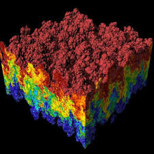Effectively we are creating an ecosystem where the apex predators are missing, and this isn’t a good thing. The models we use in science are the key to everything. They are the translation of our understanding into mathematics that we can solve and manipulate to explore our collective reality. Computers allow us to solve much more elaborate models than otherwise possible, but little else. The core of the value in scientific computing are the capacity of the models to explain and examine the physical World we live in. They are the “apex predators” in the scientific computing system, and taking this analogy further our models are becoming virtual dinosaurs where evolution has ceased to take place. The models in our codes are becoming a set of fossilized skeletons and not at all alive, evolving and growing.

The process of our models becoming fossilized is a form of living death. Models need to evolve, change, grow or even become extinct for science to be healthy. In the parlance of computing, models are embedded in codes and form the basis of a code’s connection to reality. When a code becomes a legacy code, the model(s) in the code become legacy as well. A healthy ecosystem would allow for the models (codes) to confront reality and come away changed in substantive ways including evolving, adapting and even dying as a result. In many cases the current state of scientific computing with its focus on HPC does not serve this purpose. The forces that change codes are diverse and broad. Being able to run codes at scales never before seen should produce outcomes that sometimes lead to a code’s (model’s) demise. The demise or failure of models is an important and health part of an ecosystems missing today.

People do not seem to understand that faulty models render the entirety of the computing exercise moot. Yes, the computational results may be rendered into exciting and eye-catching pictures suitable for entertaining and enchanting various non-experts including congressmen, generals, business leaders and the general public. These eye-catching pictures are getting better all the time and now form the basis of a lot of the special effects in the movies. All of this does nothing for how well the models capture reality. The deepest truth is that no amount of computer power, numerical accuracy, mesh refinement, or computational speed can rescue a model that is incorrect. The entire process of validation against observations made in reality must be applied to determine if models are correct. HPC does little to solve this problem. If the validation provides evidence that the model is wrong and a more complex model is needed then HPC can provide a tool to solve it.

The modern computing environment whether seen in a cell phone, or a supercomputer is a marvel of the modern World. It requires a host of technologies working togetherseamlessly to produce incredible things. We have immensely complex machines that produce important outcomes in the real world through a set of interweaved systems that translate electrical signals into instructions understood by the computer and humans, into discrete equations, solved by mathematical procedures that describe the real world and ultimately compared with measured quantities in systems we care about. If we look at our focus today, the complexity of focus is the part of the technology that connects very elaborate complex computers to the instructions understood both by computers and people. This is electrical engineering and computer science. The focus begins to dampen in the part of the system where the mathematics, physics and reality comes in. These activities form the bond between the computer and reality. These activities are not a priority, and conspicuously diminished significantly by today’s HPC.

HPC today is structured in a manner to eviscerate fields that have been essential to the success of scientific computing. A good example is our applied mathematics programs. In many cases applied mathematics has become little more than scientific programming and code development. Far too little actual mathematics is happening today, and far too much focus is seen in productizing mathematics in software. Many people with training in applied mathematics only do software development today and spend little or no effort in doing analysis and development away from their keyboards. It isn’t that software development isn’t important, the issue is the lack of balance in the overall ratio of mathematics to software. The power and beauty of applied mathematics must be harnessed to achieve success in modeling and simulation. Today we are simply bypassing this essential part of the problem to focus on delivering software products.

Similar issues are present with applied physics work. A healthy research environment for making progress in HPC would see far greater changes in modeling. A key aspect of modeling is the presence of experiments that challenge the ability of modeling to produce good useful representations of reality. Today such experimental evidence is sorely lacking and significantly hampered by the inability to take risks and push the envelope with real things. If we push the envelope on things in the real world it will expose our understanding to deep scrutiny. Such scrutiny will necessitate changes to our modeling. Without this virtuous cycle the drive to improve is utterly lacking.

Another missing element in the overall mix is the extent to which modeling and simulation supports activities pushing society forward. We seem to be in an era where society is not interested in progressing at anything these days. Instead we are trying to work toward a risk free world where everyone is completely safe and entirely divorced from ever failing at anything. Because of this environment the overall push for better technology is blunted to the degree that nothing of substance ever gets done. The maxim of modern life is that vast amounts of effort will be expended to assure that trivially possible things are assured of not happening. No small possibility of a dire outcome is too small to inhibit the expenditure of vast resources to make this smaller. This explains so much of what is wrong with the World today. We will bankrupt ourselves to achieve many expensive and unimportant outcomes that are completely unnecessary. Taking this view of the World allows us to explain to utter stupidity of the HPC world.

The origin, birth and impact of modeling and simulation arises from its support of activities essential to making societal progress. Without activities working toward societal progress (or at least the scientific-technological aspects of this) modeling and simulation is stranded in stasis. Progress in modeling and simulation is utterly tied to work in areas where big things are happening. High performance computing arose to prominence as a tool to allow modeling and simulation to tackle problems of greater complexity and difficulty. That said HPC is only one of the tools allowing this to happen. There is a complex and vast chain of tools necessary for modeling and simulation to succeed. It is arguable that HPC isn’t even the most important or lynchpin tool in the mix. If one looks at the chain of things that needs to work together the actual computer is the farthest removed from the reality we are aiming to master? If anything along the chain of tools closer to reality breaks, the computer is rendered useless. In other words, the computer can work perfectly and be infinitely fast and efficient, yet still be useless unless the software running on it is correct. Furthermore in the exercise of modeling and simulation, the software must be based on firm mathematical and physical principles, or it will be similarly useless. This last key step is exactly the part of the overall approach we are putting little or no effort in to in our current approach. Despite this lack of evidence we have made HPC central to success today. Too much focus on a tool of limited importance will swallow resources that could have been expended on more impactful activities. Ultimately the drivers for progress at a societal level are necessary for any of this work to have actual meaning.

If I’m being honest modeling and simulation is just a tool as well. As a tool it is much closer to the building of something great than the computers are. Used properly it can have a much greater impact on the capacity for helping produce great things than the computers can. What we miss more than anything is the focus on achieving great things as a society. We are too busy trying to save ourselves from a myriad of minute and vanishing threats to our safety. As long as we are so unremittingly risk adverse we will accomplish nothing. Our focus on big computers over big achievements is just a small reflection of this vast societal ill.

To the man who only has a hammer, everything he encounters begins to look like a nail.

― Abraham H. Maslow

 

 

Good judgment comes from experience, and experience – well, that comes from poor judgment.

― A.A. Milne

To avoid the sort of implicit assumption of ZERO uncertainty one can use (expert) judgment to fill in the information gap. This can be accomplished in a distinctly principled fashion and always works better with a basis in evidence. The key is the recognition that we base our uncertainty on a model (a model that is associated with error too). The models are fairly standard and need a certain minimum amount of information to be solvable, and we are always better off with too much information making it effectively over-determined. Here we look at several forms of models that lead to uncertainty estimation including discretization error, and statistical models applicable to epistemic or experimental uncertainty.

Maturity, one discovers, has everything to do with the acceptance of ‘not knowing.

― Mark Z. Danielewski

For discretization error the model is quite simple where is the mesh converged solution, is the solution on the mesh and is the mesh length scale, is the (observed) rate of convergence, and is a proportionality constant. We have three unknowns so we need at leastmeshes to solve the error model exactly or more if we solve it in some sort of optimal manner. We recently had a method published that discusses how to include expert judgment in the determination of numerical error and uncertainty using models of this type. This model can be solved along with data using minimization techniques including the expert judgment as constraints on the solution for the unknowns. For both the over- or the under-determined cases different minimizations one can get multiple solutions to the model and robust statistical techniques may be used to find the “best” answers. This means that one needs to resort to more than simple curve fitting, and least squares procedures; one needs to solve a nonlinear problem associated with minimizing the fitting error (i.e., residuals) with respect to other error representations.

For extreme under-determined cases unknown variables can be completely eliminated by simply choosing the solution based on expert judgment. For numerical error an obvious example is assuming that calculations are converging at an expert-defined rate. Of course the rate assumed needs an adequate justification based on a combination of information associated with the nature of the numerical method and the solution to the problem. A key assumption that often does not hold up is the achievement of the method’s theoretical rate of convergence for realistic problems. In many cases a high-order method will perform at a lower rate of convergence because the problem has a structure with less regularity than necessary for the high-order accuracy. Problems with shocks or other forms of discontinuities will not usually support high-order results and a good operating assumption is a first-order convergence rate.

To make things concrete let’s tackle a couple of examples of how all of this might work. In the paper published recently we looked at solution verification when people use two meshes instead of the three needed to fully determine the error model. This seems kind of extreme, but in this post the example is the cases where people only use a single mesh. Seemingly we can do nothing at all to estimate uncertainty, but as I explained last week, this is the time to bear down and include an uncertainty because it is the most uncertain situation, and the most important time to assess it. Instead people throw up their hands and do nothing at all, which is the worst thing to do. So we have a single solution at and need to add information to allow the solution of our error model, . The simplest way to get to an solvable error model is to simply propose a value for the mesh converged solution, , which then can be used to provide an uncertainty estimate,    |A – multiplied by an appropriate safety factor .

This is a rather strong assumption to make. We might be better served by providing a range values for either the convergence rate of the solution itself. In this way we provide a bit more deference in what we are suggesting as the level of uncertainty, which is definitely called for in this case since we are so information poor. Again the use of an appropriate safety factor is called for, on the order of 2 to 3 in value. From statistical arguments the safety factor of 2 has some merit while 3 is associated with solution verification practice proposed by Roache. All of this is strongly associated with the need to make an estimate in a case where too little work has been done to make a direct estimate. If we are adding information that is weakly related to the actual problem we are solving, the safety factor is essential to account for the lack of knowledge. Furthermore we want to enable the circumstance where more work in active problem solving will allow the uncertainties to be reduced!

A lot of this information is probably good to include as part of the analysis when you have enough information too. The right way to think about this information is as constraints on the solution. If the constraints are active they have been triggered by the analysis and help determine the solution. If the constraints have no effect on the solution then they are proven to be correct given the data. In this way the solution can be shown to be consistent with the views of the expertise. If one is in the circumstance where the expert judgment is completely determining the solution, one should be very wary as this is a big red flag.

Other numerical effects need models for their error and uncertainty too. Linear and nonlinear error plus round-off error all can contribute to the overall uncertainty. A starting point would be the same model as the discretization error, but using the tolerances from the linear or nonlinear solution as . The starting assumption is often that these are dominated by discretization error, or tied to the discretization. Evidence in support of these assumptions is generally weak to nonexistent. For round-off errors the modeling is similar, but all of these errors can be magnified in the face of instability. A key is to provide some sort of assessment of their aggregate impact on the results and not explicitly ignore them.

Other parts of the uncertainty estimation are much more amenable to statistical structures for uncertainty. This includes the type of uncertainty that too often provides (wrongly!) the entirety of uncertainty estimation, parametric uncertainty. This problem is a direct result of the availability of tools that allow the estimation of parametric uncertainty magnitude. In addition to parametric uncertainty, random aleatory uncertainties, experimental uncertainty and deep model form uncertainty all may be examined using statistical approaches. In many ways the situation is far better than for discretization error, but in other ways the situation more dire. Things are better because statistical models can be evaluated using less data, and errors can be estimated using standard approaches. The situation is dire because often the issues being radically under-sampled are reality, not the model of reality simulations are based on.

Uncertainty is a quality to be cherished, therefore – if not for it, who would dare to undertake anything?

― Villiers de L’Isle-Adam

In the same way as numerical uncertainty, the first thing to decide upon is the model. A standard modeling assumption is the use of the normal or Gaussian distribution as the starting assumption. This is almost always chosen as a default. A reasonable blog post title would be “The default probability distribution is always Gaussian”. A good thing for a distribution is that we can start to assess it beginning with two data points. A bad and common situation is that we only have a single data point. Thus uncertainty estimation is impossible without adding information from somewhere, and an expert judgment is the obvious place to look. With statistical data and its quality we can apply the standard error estimation using the sample size to scale the additional uncertainty driven by poor sampling, where is the number of samples.

There are some simple ideas to apply in the case of the assumed Gaussian and a single data point. A couple of reasonable pieces of information can be added, one being an expert judged standard deviation and then by fiat making the single data point the mean of the distribution. A second assumption could be used where the mean of the distribution is defined by expert judgment, which then defines the standard deviation,  |A – where is the defined mean, and is the data point. In these cases the standard error estimate would be equal to where . Both of these approaches have the strengths and weaknesses, and include the strong assumption of the normal distribution.

In a lot of cases a better simple assumption about the statistical distribution would be to use a uniform distribution. The issue with the uniform distribution would be identifying the width of the distribution. To define the basic distribution you need at least two pieces of information just as the normal (Gaussian) distribution. The subtleties are different and need some discussion. The width of a uniform distribution is defined by – . A question is how representative a single piece of information would actually be? Does one center the distribution about ? One could be left with needing to add two pieces of information instead of one by defining and . This then allows a fairly straightforward assessment of the uncertainty.

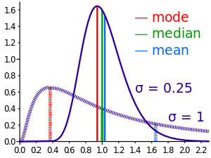For statistical models eventually one might resort to using a Bayesian method to encode the expert judgment in defining a prior distribution. In general terms this might seem to be an absolutely key approach to structure the expert judgment where statistical modeling is called for. The basic form of Bayes theorem is where is the probability of given , is the probability of and so on. A great deal of the power of the method depends on having a good (or expert) handle on all the terms on the right hand side of the equation. Bayes theorem would seem to be an ideal framework for the application of expert judgment through the decision about the nature of the prior.

The mistake is thinking that there can be an antidote to the uncertainty.

― David Levithan

A key to this entire discussion is the need to resist the default uncertainty of ZERO as a principle. It would be best if real problem specific work were conducted to estimate uncertainties, the right calculations, right meshes and right experiments. If one doesn’t have the time, money or willingness, the answer is to call upon experts to fill in the gap using justifiable assumptions and information while taking an appropriate penalty for the lack of effort. This would go a long way to improving the state of practice in computational science, modeling and simulation.

Children must be taught how to think, not what to think.

― Margaret Mead

Rider, William, Walt Witkowski, James R. Kamm, and Tim Wildey. “Robust verification analysis.” Journal of Computational Physics 307 (2016): 146-163.