While this might seem to be a bold statement, I’ll bet a lot of my colleagues would agree with this. We are as a nation destroying an incredible national resource though systematic and pervasive mismanagement. In fact, it would be difficult to conceive of a foreign power doing a better job of killing the Labs than we are doing to ourselves (think of the infamous circular firing squad).
Who is to blame?
You, and me and those who represent you in government are doing this. Both the legislative and executive branches of government are responsible along with the scandal-mongering media-political machine. The loss of anything that looks like the traditional fourth-estate helps to fuel the destruction. Our new media has now simply turned into an arm of the corporate propaganda machine mostly devoted to the accumulation of ever-greater amounts of wealth. All the responsible adults seem to have left the room. At the Labs, no amount of expense or additional paperwork will be spared to avoid the tinge of scandal or impropriety. Most of the rules taken by alone seem to be reasonable and at least have reasonable objectives, but taken as a whole represent a lack of trust that is strangling the good work that could be happening.
There are no big projects or plans that we are working on. Our Nation does not have any large goals or objectives that we are striving for. Aside from the ill constructed and overly wasteful “war on terror”, we have little or nothing in the way of vision. In truth, the entire war on terror is simply a giant money pit that supplies the military-industrial complex with wealth in lieu of the Cold War. The work at the Labs is now a whole bunch of disconnected projects from a plethora of agencies with no common theme, or vision to unite the efforts. As a result, we cost a fortune and do very very little of real lasting value any more.
More than simply being expensive and useless, something even worse has happened. We have lost the engine of innovation in the process. The vast majority of innovation is simply the ingenious application of old ideas in new contexts. The goals that served to create our marvelous National Labs served as engines of innovation because the projects required a multitude of disciplines to be coordinated engaged and melded together to achieve success. As a result of this unified purpose engineers, physicists, chemists, mathematicians, metallurgists, and more had to work together to a common goal. Ideas that had matured in one field had to be communicated to another field. Some of the scientists took this as inspiration to apply the ideas in new ways in their field. This was the engine of innovation. The core of our current economic power can be traced to these discoveries.
We are literally killing the goose that laid the golden egg, if it isn’t already dead.
Gone are bold explorations of science, and grand creations in the name of the National interest. These have been replaced by caution, incrementalism, and programs that are largely a waste of time and effort. Programs are typically wildly overblown, when in fact they represent a marginal advance. Washington DC has created this environment and continue to foster, fertilize and plant new seeds of destruction with each passing year.
Take for example their latest creation, the unneeded oversight of conference attendance. I’ll remind you that a couple of year’s ago the IRS had a conference in Las Vegas that had some events, and activities that were of questionable value and certainly showed poor judgment. What would be the proper response? Fire the people responsible. What is the government’s response? Punish everybody and create a brand new beauracracy to scrutinize conference attendance. Everyone includes the National Labs, and any scientific meetings that we participate in. The entire system now costs much more and produces less value.
All of this stupidity was done in the name of an irrational fear of scandal. The political system is responsible because one party is afraid that the other party will make political hay over the mismanagement. The party of anti-government will make an example of the pro-government party as being wasteful. No one bats an eyelash at wasting money to administer cost controls instead of spending money to actually do our mission. As a result we waste even more money while getting less done. A lot is made of applying best business practices in how we run the Labs. I will guarantee to you that no business would treat its visitors or host meetings as cheaply and disrespectfully as we do. Instead of hosting visitors in a reasonable and respectful way, we make them pay for their own meals, and hold ridiculously Spartan receptions. Only under the most extreme circumstances would a single drop of alcohol be served to a visitor (and only after copious paperwork has been pushed along). All in the name of saving money while in the background we waste enormous amounts of money managing everything we do.
I can guarantee you that our meetings are not fun; they are full of long, incomprehensible talks, terrible travel, and crappy hotels (flying coach is awful domestically, and horrible overseas). Travelling these days sucks, and I don’t like being away from my family and home. I go to meetings to learn about what my field, present my own work, and engage with my colleagues. My field is international as are most scientific disciplines. Where I work the conference attendance “tool” assumes that the only valid reason to go is to present your own work, and sometimes this reasoning doesn’t suffice. I’ll invite the reader to do the exercise of what happens if everyone just goes to a meeting to talk and not listen. What happens to the audience? Who are you talking to? Welcome to the version of science being created, it is utterly absurd. Increasingly it is ineffective.
A big part of the issue is the misapplication of a business model to science at the Laboratory. Government in the last 30 years has fallen in love with business. Business management can do no wrong, and its been applied to science. Now we have quarterly reports, and business plans. Accounting has chopped our projects into smaller and smaller pieces all requiring management and reporting. All my time is supposed to accounted for and charged appropriately to a “sponsor”. Sometimes people even ask for a project to charge for their attendance at a seminar, professional training, reviewing papers, and numerous other tasks that used to be under the broad heading of professional responsibilities. A lot of these professional responsibilities are falling by the wayside. I’ve noticed that increasingly the Labs are missing any sense of community or common purpose. In the past, the Labs formed a community with an overarching goal and reason for existence.
Now we have replaced this with a phalanx of sponsors who simply want the Labs to execute tasks, and have no necessary association with each other. It has become increasingly difficult to see any difference between the Labs and a typical beltway bandit (think SAIC, Booz-Allen, …). Basically, the business model of management has been poisonous to the Labs. Aside from executive bonuses and stock options it is arguable that the modern business model isn’t good for business either. Lots of companies are being hollowed out and having their future’s destroyed in the service of the next quarterly report. For science it is a veritable cancer, and death sentence.
On top of this it is expensive and horribly inefficient, I cost an arm and a leg, while actually producing much less output than the same scientist would have produced 30 or 40 years ago. The bottom line, the business model for scientific management is a bad deal for everyone.
As I mentioned in an early post, I think a large part of the problem is trust, or the lack thereof. Back in the days of the Cold War (before 1980), the Labs were trusted. The Nation said, “build us a nuclear stockpile” and the Labs produced. The Nation said, “let’s go to the Moon” and we went. We created an endless supply of technology and science as a collateral effect of this trust. In those days the money flowed into the Labs in very large chunks (on the order of a billion current dollars), with broad guidance of what needed to be achieved (build weapons, go to the moon, etc…). The Labs were trusted to divvy up the money to tasks needed to execute the work and produce the desired outcome. It worked great, and the Nation received a scientific product that massively exceeded the requested outcomes. In other words, we got more than we asked for.
Now, we get less, and in fact because of the fear of failure what the Labs promise is a severely “low balled”. The whole thing revolves around the issue of trust, and the impact of the lack of trust in the modern world. A big part of what the Labs used to create was driven by serendipity, where new ideas arose through the merging of old ideas associated with the differing disciplines brought together to execute those Cold War missions. Now the missions are largely gone because the nation seems to lack any sense of vision, and the work is parceled out in small chunks that short-circuit the interactions that drive the serendipity. No larger vision or goal binds the work at the Labs together, and drives the engine of innovation.
What has and is happening is a tragedy. Our National Labs were marvelous places. They are now being swallowed by a tidal wave of mediocrity. Suspicion and fear are driving behaviors that hurt our ability to be a vibrant scientific Nation. The Labs were created by faith and trust in the human capacity for success. They created a wealth of knowledge and innovation that enriches our Nation and World today.
It is time to stem the tide. It is time to think big again. It is time to trust our fellow citizens to do work that is high-minded. It is time to let the Labs do work that is in the best interest of the Nation (and humanity).
 .
.
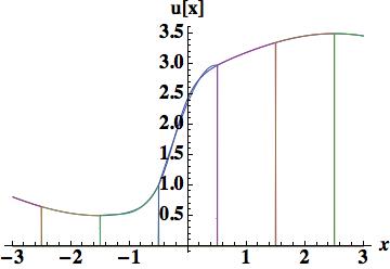
 , which is the foundation of Godunov’s method, a first-order, but monotone method. The integrated difference between the analytical function and this piecewise polynomial is 0.882015, which will serve as a nice measure of success with higher order reconstructions.
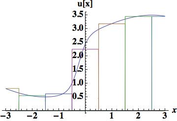
 . The improvement over the piecewise constant is obvious and the integrated error is now, 0.448331 about half the size of the piecewise constant.
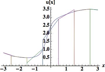
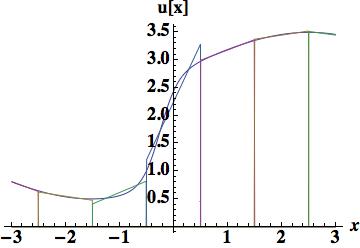
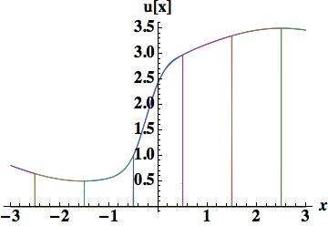
 . We stay with Van Leer’s use of Legendre polynomials because they are mean preserving without difficulty. The first is the parabola determined by the three centered cell center values, which gives a relatively large error of 0.427028 almost as large as the piecewise linear interpolation.

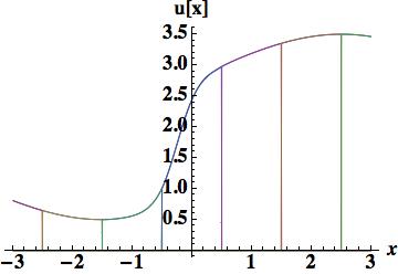
 . We will look at two reconstructions, the first based on three cell-centers, and an integral of the derivative in the center cell. This is a Hermite scheme, and based on previous experience with Schemes 1 and 4 we should expect its performance to be relatively poor with an error of 0.14884, one-third of that found with the piecewise parabolic scheme 4. The second cubic reconstruction will use the cell-center, edges and the first moment, provides excellent results, 0.044014 approximately on par with the two moment piecewise parabola the basis of scheme 6. The method to update the degrees of freedom is arguably simpler (and the overall degrees of freedom is equivalent).
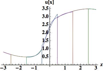
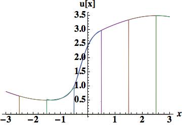
 . Four different methods will be used to determine the coefficients. The first is a fairly important approach because the evaluation provides the stencil used for the upstream-centered fifth order WENO flux. This polynomial is determined by the cell-centered values in the cell and the two cells to the left or right. The figure shows that the polynomial is relatively poor in terms of accuracy, and confirmed by the integrated error, 0.404114 barely better than the parabola used for scheme 4. The quartic reconstruction must provide greater value.
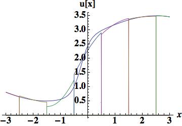

 . Five cell-center values participate in the scheme,
  . The standard approach then derives parabolic approximations based on stencil using cells,
  ,
,  , and
, and  . By some well-defined means the smoothest stencil among the three is chosen to update
  ,
,  , and
, and  . Weights are defined by using the derivatives of the corresponding parabolas to measure the smoothness of each. The weights are chosen so that in smooth regions the weights give a fifth-order approximation to the edge value,
  . The point is that the same principles could be used for other schemes, indeed they already have been in the case of Hermitian WENO methods.
 ,
,  and
and  . This gives a parabola of
 .
. .
. and
and  .
. .
. ,
,  .
. .
. and cell-edge values,
  . This defines a quartic polynomial,


 .
. . This is exceedingly accurate with the dispersion relation peaking at
  with an error of only 2.5%.
 , and the edge-first-derivatives,
  .It is also similar to the PQM method proposed for climate studies. The PQM method is implemented much like PPM in that the edge variables are approximated in terms of the cell-centered degrees of freedom. Here we will describe these variables as independent degrees of freedom. The polynomial reconstruction defined by these conditions is


 .
. . This is exceedingly accurate with the dispersion relation peaking at $latex\theta=\pi$ with an error of only 1.2%.
 .
. .
.

 .
. . This is exceedingly accurate with the dispersion relation peaking at $latex\theta=\pi$ with an error of only 3.1%.

 .
. . This is accurate with the dispersion relation peaking at $latex\theta=\pi$ with an error about 12%.

 .
. . This is accurate with the dispersion relation peaking at $latex\theta=\pi$ with an error of 10%. The last two methods may not be particularly interesting in and of themselves, but may be useful as alternative stencils for ENO-type methods.
 or
or 
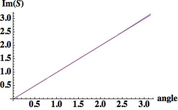
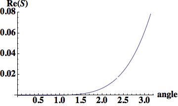
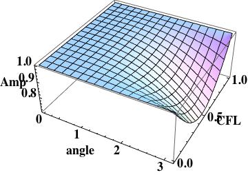
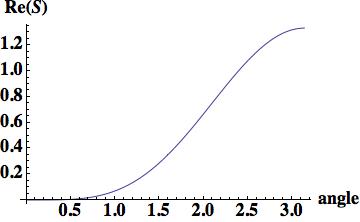
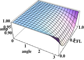
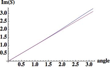
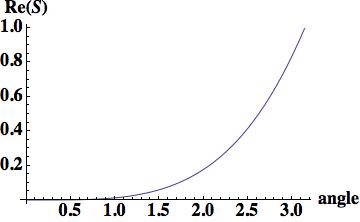
 being the angle and
  being the amplification factor.
 with
with  ,
,  with slopes computed from local data
  .
.
 and
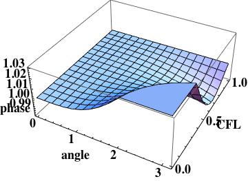
and  is the CFL number.
 .
.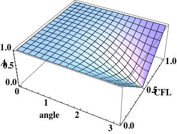

 this is the leading order error (being one order higher due to how the phase error is written). A key aspect of this scheme has zero phase error at CFL numbers of one-half and one.
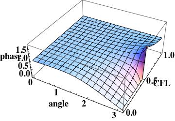
 , which is useful if the scheme is used with a method-of-lines time integration.
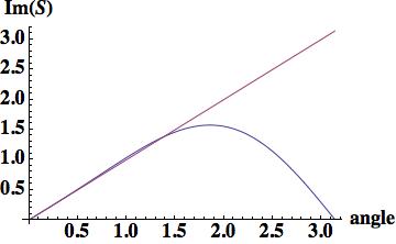

 in time. The update is then two equations, one for the cell-centered data,
 ,
, ,
, as the initial slope is replaced by the first expression on the right hand side of the equation driving a coupling of the variable and the slope in the update.
 .
.
 and is the leading order error as with all of the first three methods. Again, this method does not lend itself to a well-defined semi-discrete method.
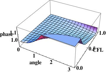
 , but
, but  . Here, as with Scheme II, we evolve both
  , and
, and  , but the evolution equation for
  ,
, ![\partial_t m - \int_{-1/2}^{1/2} \partial_x \xi u d\xi + [u(1/2)+u(-1/2)] = 0](https://s0.wp.com/latex.php?latex=%5Cpartial_t+m+-+%5Cint_%7B-1%2F2%7D%5E%7B1%2F2%7D+%5Cpartial_x+%5Cxi+u+d%5Cxi+%2B+%5Bu%281%2F2%29%2Bu%28-1%2F2%29%5D+%3D+0&bg=ffffff&fg=000&s=0&c=20201002) .
. , where
  .
. .
.
 now the amplification error is leading and the method is confirmed as being third-order. This scheme is obviously more accurate than the previous two methods.
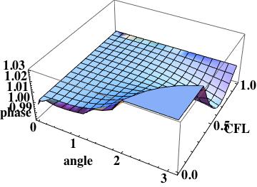
 , which the keen observer will notice being third-order accurate instead of the expected second order. Van Leer made a significant note of this.

 ,
, , and
, and  . This is a third-order method.
 . The update then is simply the standard conservative variable form,
 .
.

 this is the leading order error (being one order higher due to how the phase error is written). A key aspect of this scheme has zero phase error at CFL numbers of one-half and one.
 , which is useful if the scheme is used with a method-of-lines time integration.
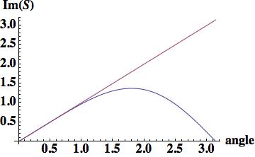
 and the value at the edges
  . The coefficients are then simply defined by
  , and
, and  . This is a third-order method.
 ,
, .
.
 .
.
 .
. ,
,  , and
, and 
 .
.  is the first moment of the solution, and
  is the second moment. The moments are computed by integrating the solution multiplied by the coordinate over the mesh cell. This is a fifth-order method.
 , which the keen observer will notice being fifth-order accurate instead of the expected third order. The semi-discrete update for the first moment is
  , and the second moment is
 .
.