tl;dr

In CFD computing, a stable time step size is fundamental to explicit methods. To do this, accurate wave speeds are needed. Wave speeds are important for (approximate) Riemann solvers or artificial dissipation settings. Classical methods evaluate the wave speeds from static data at the beginning of a time step. Dynamics in a problem can change these wave speeds significantly. In some cases, the increase in speed can be far larger than realized commonly. Under estimates result in violating linear and nonlinear stability conditions as well as entropy conditions. These violations are subtle and manifest themselves in unusual ways. We suffer from focus on shock and have ignored expansions to our detriment.

“The biggest wave is the one that comes from where you least expect it!” ― Mehmet Murat ildan

Recap from void problems

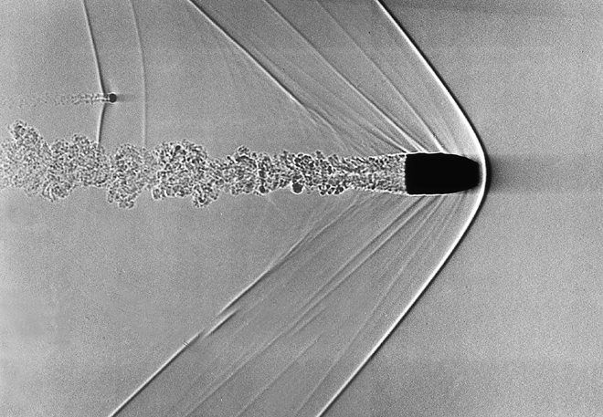
As a starting point we can do a brief summary of the void problems that inspired all this. Sandia (and other places) codes introduce void into their problems to avoid issues usually with equations of state. These voids then offer a place for material to expand into. It turns out that expansion to void is a very hard problem for hydro codes. The answers it produces are quite bad too. In the case of the code I was examining, the initial problem produced a catastrophic collapse of the calculation. When abstracting to a simple 1-D problem, the code produced poor answers that converged very slowly to the correct solution, if at all. The instability in the calculation seems to be a multidimensional effect. The mesh required for good solutions is ridiculous. There needs to be a better way forward.

“Without boundaries you are lost in the void with no horizon.” ― Elena Tauros

In order to look for ways to solve this problem correctly, I looked at other codes and methods. These codes are based on more solid principles, and I expected better results. This did not happen. The problem appears to be a pox on all hydrocodes. I started to look at the problem in detail and examined all manner of variation in the methods. Nothing worked to cure the issues. Some things made matters worse. Riemann solvers were not the cure. Higher order methods were not the answer. WENO (or ENO) was not. A host of modern methods considered standard or better failed to solve things. Excess dissipation made things worse too. There is something much deeper at the bottom of this.

A core issue is that CFD codes focused on shock waves since the beginning. Expansions looked benign and not dangerous to code stability. When a shock formed and was not stabilized, the entire solution was threatened, and the code’s results blew up. This made is a focus for artificial viscosity and development. Shocks are exciting. When we got them working we created a whole field of shock capturing methods and CFD was born. Expansions seem to be simple and easy, until they aren’t. The expansions are details we haven’t focused much energy on and now its time to fix this. In a large class of problems these effects are important, it is time to start cleaning this up.

“Youth always tries to fill the void, an old man learns to live with it.” ― Mark Z. Danielewski

The issue of poor wave speed estimates is not the cure, but it is important. Too important to not elaborate on.

How wrong can it be?

“The wave is never alone; if there is a wave somewhere, there are other waves in front and behind!” ― Mehmet Murat ildan

One of the big things I discovered in looking at this problem is how bad standard wave speed estimates can be. I had known about this for a while. In a sense I knew about half the problem, and true to form, the half involving shock waves. I knew that as shocks grow stronger the shock speed becomes much larger than the wave speeds on either side of the wave. This can be seen in computing a shock moving from high pressure to low from stationary initial conditions. Rankine-Hugoniot conditions are algebraic and shock conditions are tractable to compute. I had added these conservative estimates to Riemann solvers, and time step size considerations in all my codes.

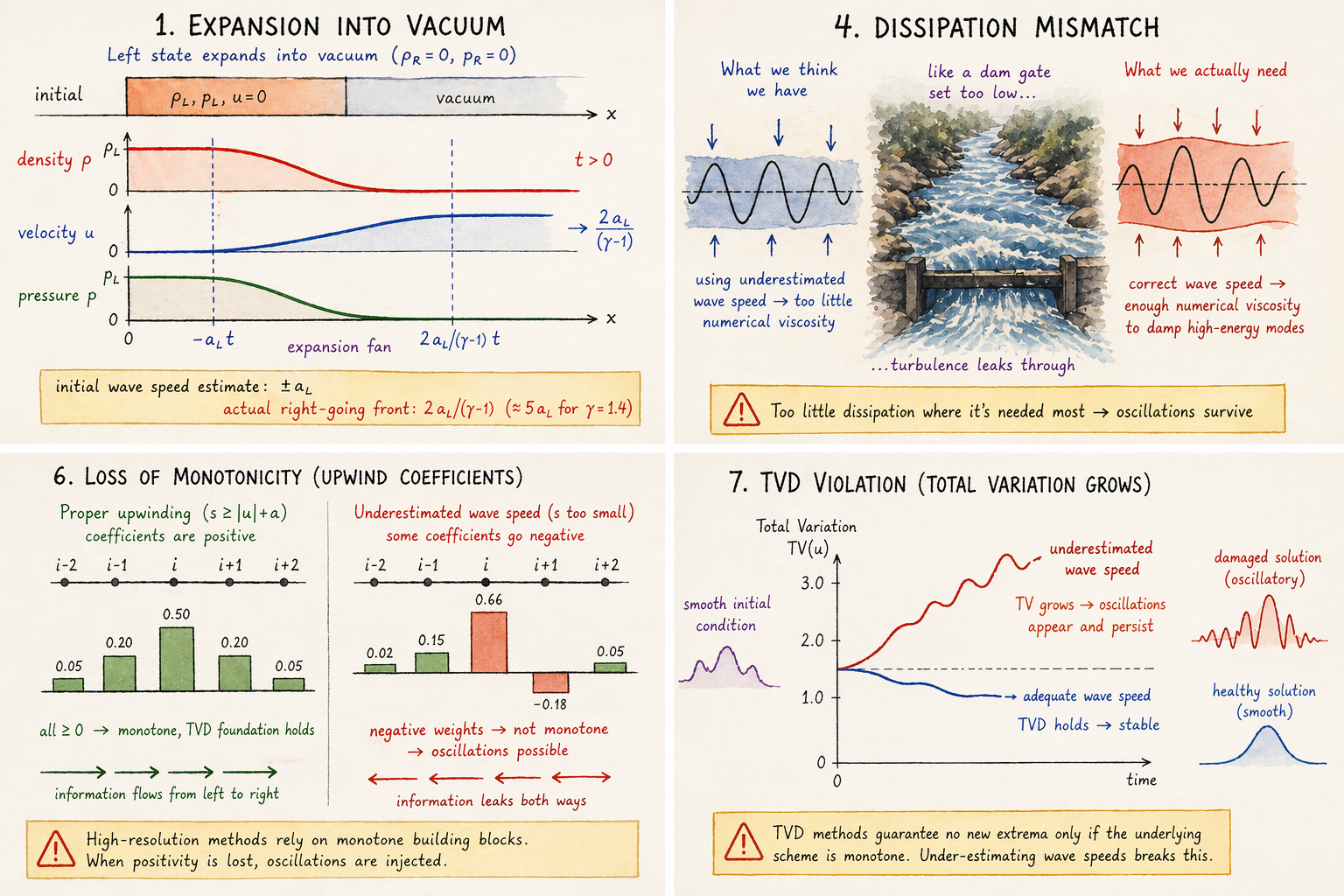
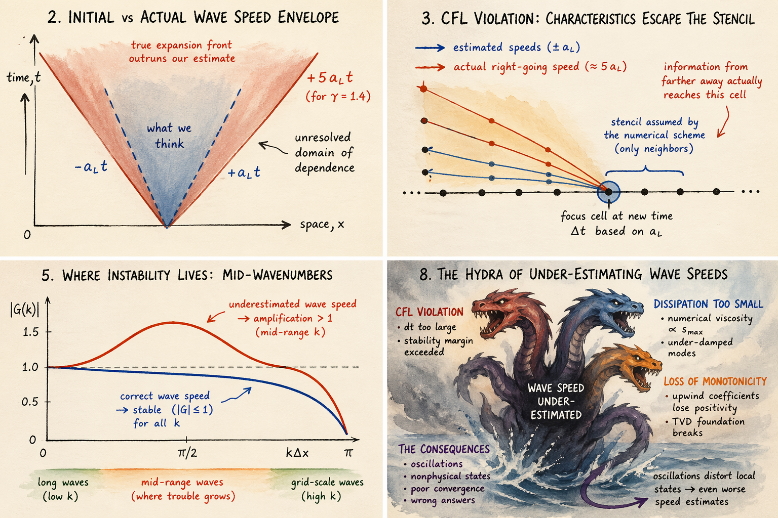
What I didn’t realize was how wrong the wave speeds would be in an expansion. For extreme expansions like expansion into vacuum, the waves peeds could be very fast. The difference between these waves speeds and initial conditions could be larger than an order of magnitude. Worse yet, the expansions are integral conditions and more difficult to compute and bound. Fortunately, this problem has attracted a great deal of attention in the last decade (references at the end). Some of the papers are quite challenging to read. Much of the focus is on wavespeeds for dissipation in methods. In addition, they use it to determine time steps sizes. What isn’t entirely clear is the penalties for not doing this.

“You never really know what’s coming. A small wave, or maybe a big one. All you can really do is hope that when it comes, you can surf over it, instead of drown in its monstrosity.” ― Alysha Speer

These are potentially quite severe, but also not as bad a one might fear. It isn’t clear whether any of this is associated with the convergence issues afoot in the extreme expansions. I’m about to elaborate on all this.

What’s at stake?

“Stability. The primal and ultimate need. Stability. Hence all this.” ― Aldous Huxley

If one consults the literature and asks how does one determine the time step size?

The answer is usually “linearize the equations and compute the eigenvalues of the flux Jacobian”. For the Euler equations this gives the velocity and the acoustic eigenvalues with velocity plus or minus the sound speed. These are evaluated from initial conditions. As noted above dynamics of the Euler equations produce wave speeds that are far larger. Ad hoc methods are used to deal with this. First, one applies a safety factor to the time step size. With initial conditions, the time step is often slowly ramped up. A problem is that these sorts of conditions can arise dynamically as a problem evolves. This would occur without some of these remediating procedures. A good example is the collision of two shock waves (like the Woodward-Colella blast wave problem).

I will note that this could be fixed generally. If one tested the final conditions from a time step and computed a limit. Then check the time step just taken, and see if it was stable. If it is not stable then back up, throw away that time integration and do it over with a smaller time step. This would require storing an additional solution field. This is a difficult method that no one does this. Its a painful method that still might be worth the effort. It would be fun to explore this. I’m sort of amazed that no production codes do this.

“Real stability isn’t inherited. It’s engineered.” ― Shamail Aijaz

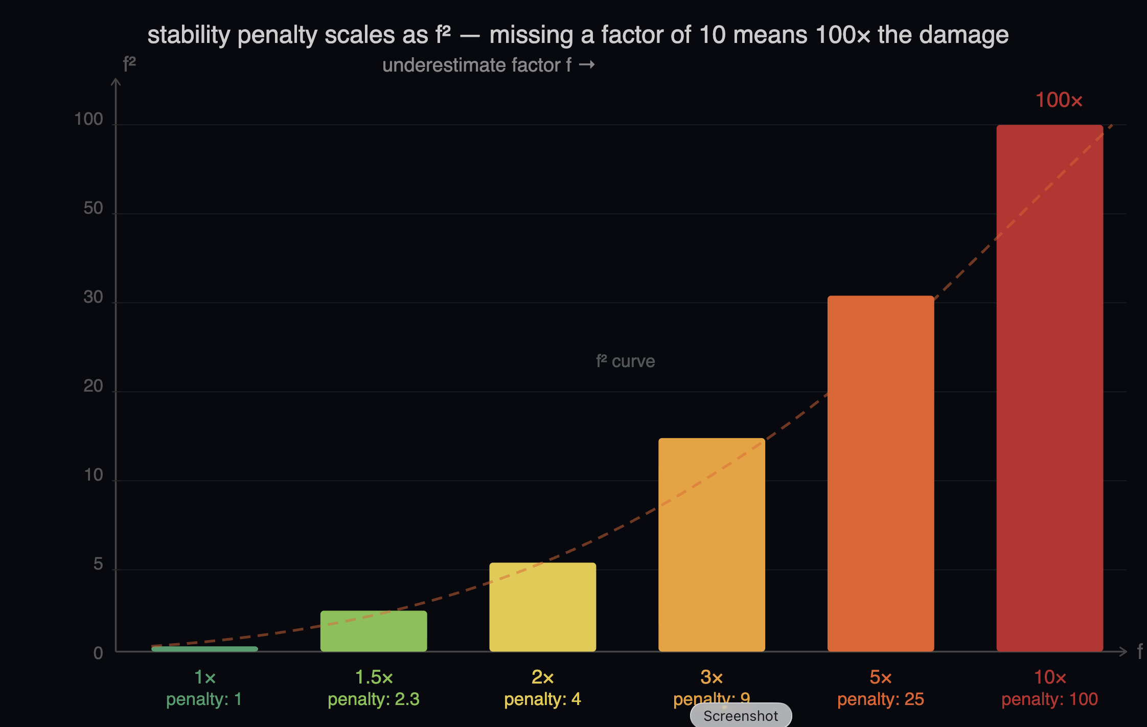
This does not get rid of all the problems. Wavespeeds are needed to properly dissipate methods to produce stability. If you have estimates that are lower, the method isn’t properly upwind. This not quite upwind method will have a lower stability limit proportional to the under-estimate. If you are taking a larger time step due to a smaller wave speed, you are also violating stability. These two effects then work together and the impact is quadratic in the underestimate. So if you miss the wave speeds by a factor of two, the effect on the stability is four times. If you miss by a factor of ten, the effect on stability is 100. Fortunately (or not), there is a saving grace.

“But what happens when there’s a ripple in the flow and it turns out to be more than you can handle?” ― Dominic Riccitello

The worst instabilities happen at high wave numbers, the grid frequency. This is the classical catastrophic numerical instability. Fortunately for the problem discussed here, the instability is at mid to low wave numbers. Its unfortunate because this has masked the problem for decades. Thus, the instability and oscillations are generated on a larger scale. This is probably why solutions are not blowing up. Nonetheless, the result is likely oscillations and solutions that survive, but are damaged. We should probably fix this in our codes. Mostly people don’t give a fuck. The code runs on a super-fast computer. The problem is that this problem can’t be escaped by a faster computer. A bigger faster computer just means you waste more money. You don’t solve the issue at all.

This issue is not done fucking us yet. If one looks at upwinding it is a monotone method. This means that it is positive in its coefficients. This positivity is the foundation of high-resolution non-oscillatory methods. This can be seen through the theory of TVD methods. If you upwind with too small a wave speed, the method is no longer monotone or positive. In addition to stability violations this is another source of oscillations. All the high resolution methods use upwind methods of some sort as a foundation. Thus this problem undermines all of these and potentially injects oscillations into the solutions. The proper and correct upwind method is the foundation of all high resolution methods. If your monotone method is wrong, nothing rescues what is build on top of it.

This problem is a veritable multi-headed hydra of effects undermining our fundamental methods. Fixing these should be essential to our codes. We have a route to improve all our most important codes. I’ve wondered why this sort of fundamental work is so difficult to get support for. It is also unlikely to fix the issues with extreme expansions, but might be part of it. If we care about fundamental issues like stability (we should) the answer is easy.

In this topic I find yet another concise reason for my decision to exit Sandia. There was so little respect for fundamentals or the experts who care for them.

“Never think that lack of variability is stability. Don’t confuse lack of volatility with stability, ever.” ― Nassim Nicholas Taleb

References

Menikoff, Ralph, and Bradley J. Plohr. “The Riemann problem for fluid flow of real materials.” Reviews of modern physics 61, no. 1 (1989): 75.

Guermond, Jean-Luc, and Bojan Popov. “Invariant domains and first-order continuous finite element approximation for hyperbolic systems.” SIAM Journal on Numerical Analysis 54, no. 4 (2016): 2466-2489.

Guermond, Jean-Luc, Murtazo Nazarov, Bojan Popov, and Ignacio Tomas. “Second-order invariant domain preserving approximation of the Euler equations using convex limiting.” SIAM Journal on Scientific Computing 40, no. 5 (2018): A3211-A3239.

Guermond, Jean-Luc, and Bojan Popov. “Fast estimation from above of the maximum wave speed in the Riemann problem for the Euler equations.” Journal of Computational Physics321 (2016): 908-926.

Toro, Eleuterio F., Lucas O. Müller, and Annunziato Siviglia. “Bounds for wave speeds in the Riemann problem: direct theoretical estimates.” Computers & Fluids 209 (2020): 104640.

Clayton, Bennett, Jean-Luc Guermond, and Bojan Popov. “Invariant domain-preserving approximations for the Euler equations with tabulated equation of state.” SIAM Journal on Scientific Computing 44, no. 1 (2022): A444-A470.

Clayton, Bennett, and Eric J. Tovar. “Preserving the minimum principle on the entropy for the compressible Euler Equations with general equations of state.” arXiv preprint arXiv:2503.10612 (2025).