“The real purpose of the scientific method is to make sure nature hasn’t misled you into thinking you know something you actually don’t know.” ― Robert M. Pirsig

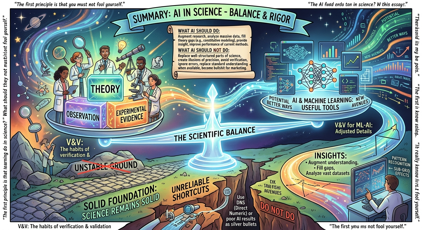
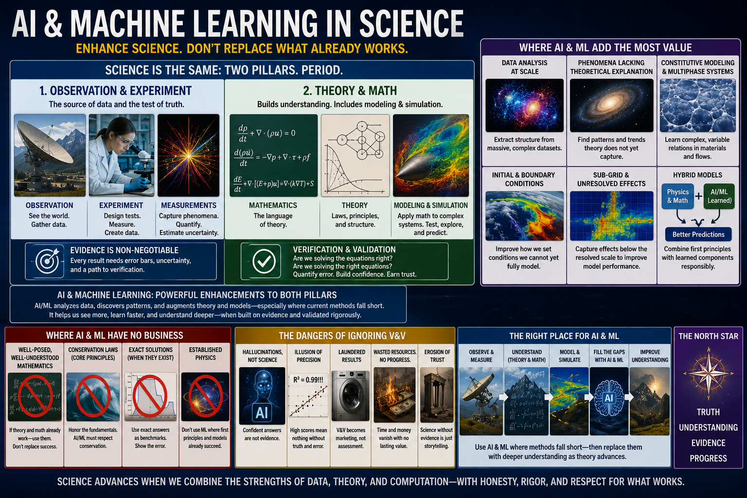
My thoughts on how machine learning (ML) fits into science are shaped by the question of how simulation fits into science. In the past, I have made my views on that clear. Modeling and simulation does not change science in any fundamental way. It is just a tool to do science better. ML or AI are the same. Useful tools for better science, but science is unchanged.

The scientific method remains solid. This is a core message: science is unchanged. You just have new tools to conduct it. These new tools offer new, potentially better ways to do the same work. They offer new avenues for engaging and improving parts of it. You still have theory and observation as the base of science. Now one has more effective and more broadly applicable computational tools to navigate that space. These new tools can apply to vast datasets produced by observations or simulations. They offer new perspectives or uses of data that could improve science.

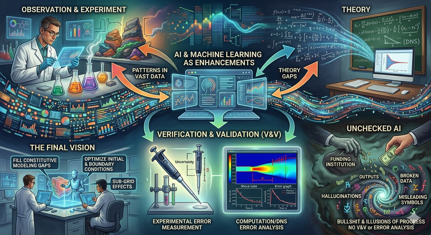
As I have said before, the key to navigating this properly is the habits and practices of verification and validation. I have argued that verification and validation are the scientific method structured for modeling and simulation. For ML and AI the same maxims apply here. For ML and AI, the details need to be sorted out differently. These techniques carry a different set of key technical practices and issues, and V&V should be adjusted accordingly. Most notably the role of theory and mathematics is fundamentally different. The math for ML-AI is vastly different and less rigorous than modeling and simulation. That is the topic I will take up in the following post in an expanded form.

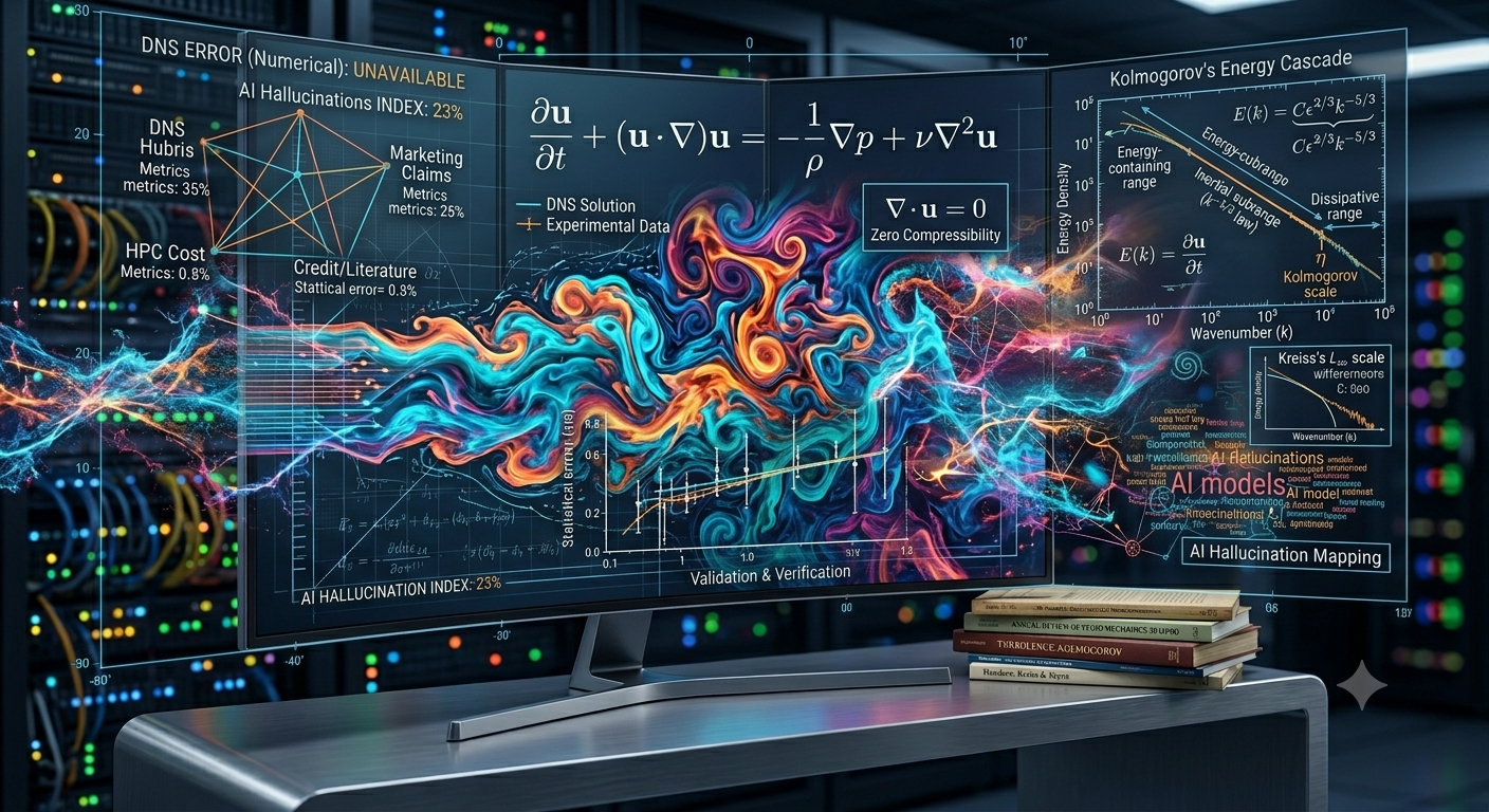
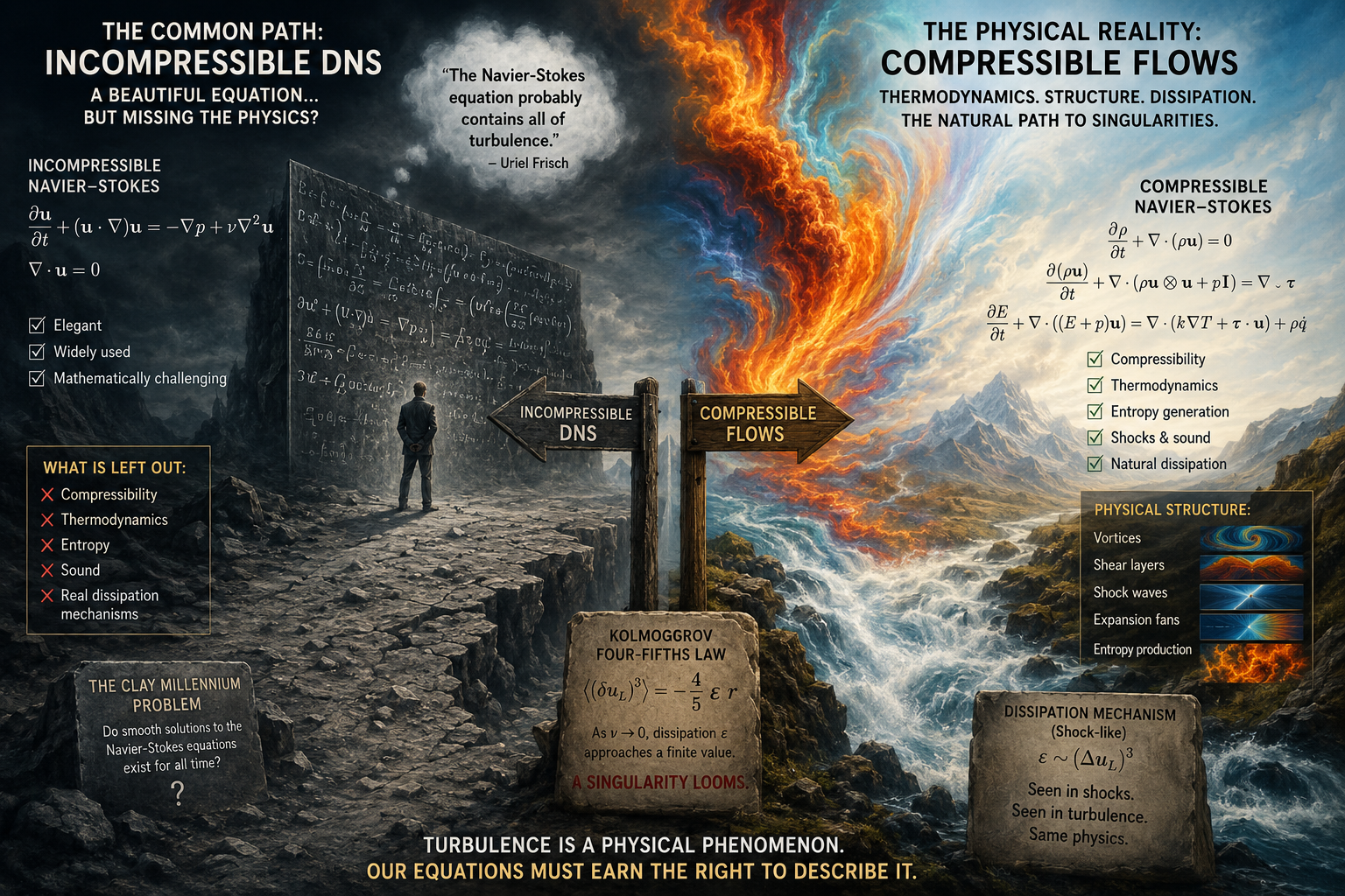
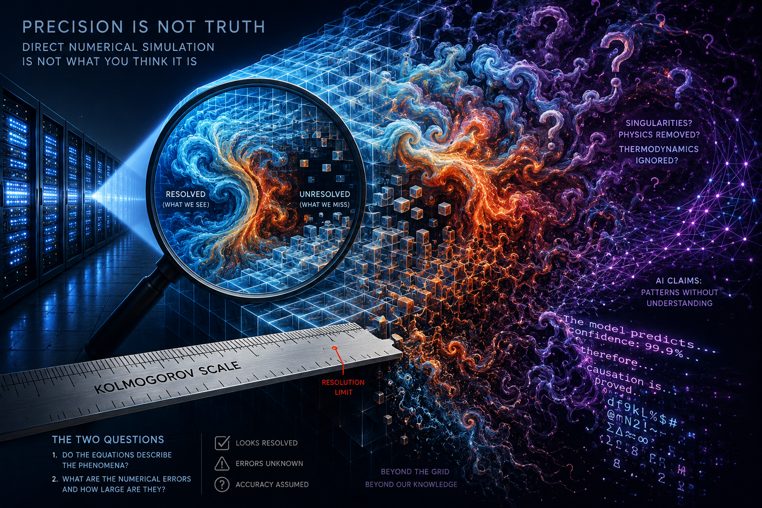
A good starting point is the subject of my last post: Direct Numerical Simulation (DNS). DNS is often promoted as the gold standard of modeling and simulation. It is supposedly so good that it can replace experimental data, which would be amazing if we could actually do it. Current practice is not up to this end. The same issue is doubly true for ML-AI. Without a great deal of improvement and better quality these won’t be silver bullets.

The history of science, like the history of all human ideas, is a history of irresponsible dreams, of obstinacy, and of error. But science is one of the very few human activities — perhaps the only one — in which errors are systematically criticized and fairly often, in time, corrected. This is why we can say that, in science, we often learn from our mistakes, and why we can speak clearly and sensibly about making progress there.” ― Karl R. Popper

That means DNS should face a very high bar for success. As I wrote, the work usually does not clear that bar. A big part of clearing the bar is entering into the sudy with doubt and uncertainty. There is typically very little analysis of whether the model equations are appropriate. Next, on whether the simulations are numerically accurate. Error analysis is at the heart of science, and that heart is largely neglected in DNS practice. ML and AI are the next fields to commit these same sins. Science is largely the study of error. Without it, the claims of science are weak.

One key question about these new tools is whether they replace parts of science that already work. Experimental and observational science remain essential to everything. They connect to objective reality. This should remain central to everything. The theory of physics, and the use of mathematics to model it, is another area where science works well. We should recognize the shortcomings in both and shore them up with new techniques. Nothing points to discarding either. As a new numerical method, or instrument improves science, AI and ML can be the same. A better tool for engaging with the same science.

AI and machine learning rely on data, which can come from observations, experiments, or simulations. it is often available in vast quantities. More with each passing year. The lack of any characterization of error and uncertainty in these data sources is one of my most consistent complaints about current practice. In almost every example I have seen, error and uncertainty are ignored rather than treated as part of training or of using these tools for science. This should be completely unacceptable, yet I see little progress toward addressing the flaw. Moreover, we should know whether the processing or use of the data expands or contracts the errors.

“Essentially, all models are wrong, but some are useful.” – George Box

One thing that is consistently missing is a commitment to evidence. This holds even for experimental data. Error is often absent or buried from the view of the consumer. This is odd as error estimation in measurement or phenomenology is well defined and expected. The standard is simply not exercised. In computation, the practice is much worse. I pointed this out for DNS, but the same is true across the field. When this happens the implicit effect is to substitute a value of zero for a true analysis. Notably, the lack of analysis and disclosure means the smallest value is used. This is intrinsically dangerous.

One area where I focus a lot of energy is the quality of shock tube solutions. These solutions are exact and come with a precise error estimate. Yet the accepted practice across the community is to not display those errors. We are offered purely qualitative results. There is little reflection on this. It is simply what I call “Hello World” for the field. It is really a quiet sad state of affairs. The result is an unconscious stagnation, where we show qualitative results, give a thumbs up or thumbs down, and move on. No evidence is provided about the error or efficiency of the methods. It is common in other parts of computational science. We see the same trend in machine learning and AI.

“Science, my boy, is made up of mistakes, but they are mistakes which it is useful to make, because they lead little by little to the truth.” ― Jules Verne

Over my career, I watched the rise of V&V, driven by the promise of doing high-consequence work with the quality and evidence that supported its use. This spirit rose and fell in less than a decade. After that, I saw roughly a 20-year pullback, as the evidence was deemed too expensive, too difficult, and insufficiently positive to power the marketing our programs needed. Evidence and doubt are essential for science. They are anathema to marketing. Our institutions are mostly marketing with very little science.

That period coincided with V&V providing genuine assessments of techniques and science. Such assessments often highlight problems and areas for further work. This powers the advance of science. It is not the success message our programs seem to require in today’s untrusting environment. As a result, V&V has largely become a way to launder results and supply the positive messaging that supports funding. This is the only thing our management and institutions seem to care about today.

AL and ML are now being added to this toxic mixture. AI and machine learning need the spirit of quality and assessment far more than modeling and simulation do, even more than DNS does. Without it, the likely outcome is an endless parade of hallucinations and bullshit. These will be presented as silver bullets for every kind of problem, while amounting to nothing more than illusions of progress. For applications and decisions of high consequence this is a disaster waiting to unfold.

Right now, everyone is lined up at the trough of money around AI and ML. They are just wanting to feed. Very little proof is needed, and even less is desired. I fear this lack of appetite for V&V is a tell about how little faith people actually have in the work, and an implicit understanding that the evidence will not be positive. Not wanting V&V, or evidence of the error structure in science, is a clear sign that, deep down, people know they are engaged in bullshit. They know that at some level V&V will expose them as liars. They are offering the illusion of precision without being willing to put up the evidence that would demonstrate it.

“The first principle is that you must not fool yourself, and you are the easiest person to fool.” – Richard Feynman

So what should ML and AI do for science, and what should they not?

The way to decide is clear: look at these new tools through the lens of the structure of science. The structure that is invariant to the tools used.

We start with experimental and observational science, then move to theory, which is often mediated through modeling and simulation. ML offers fantastic ways to augment experimental and observational science by analyzing data. This is especially available in vast quantities gathered in new ways. This path also points toward how ML can affect theory. Most notably whether there are trends or aspects of the data that currently resist structured explanation. ML offers new ways to represent and navigage poorly understood aspects of vast datasets.

The same pattern holds for modeling. There are aspects of our world that our existing models do not capture, and these gaps in current theory are exactly where the new tools can reside. In the best case, these ML results will themselves be replaced by structural understanding as much as possible. If a standard structured theory is available, ML is surplus to requirements. That is the frontier we should push on. In the end, if we gain understanding through modeling, the need forML decreases. We will always have areas we do not understand, or that are not amenable to the modeling tools we currently have,. In that sense ML can augment our understanding.

The more controversial point is where these tools have no business playing at all. I have seen plenty of papers aimed at the well-structured, well-posed mathematical parts of a system that ML is trying to replace. That strikes me as utterly ludicrous. If something is well understood, well posed, and well constructed mathematically, ML has no business operating there. It should operate where our theory and methods fail, not where they succeed.

Conservation laws are essential, but they are not always precise, and this matters for machine learning. Conservation of mass, for example, is sacrosanct. As soon as you move to the momentum or energy equations, constitutive modeling starts to play a key role. This is where ML can start to engage, That is especially true in multi-phase flow, where constitutive modeling is woven into nearly every part of the methodology. Parallels exist across different modeling problems.

ML fits into the gaps around constitutive modeling and its variations. Another such area is the setting of initial and boundary conditions for calculations. Our current methods do not fully capture these impacts. Where there are substantial sub-grid effects below the macro scale, ML and AI can help fill those gaps and improve the performance of the methods we use today. The key is to recognize where tools have the potential to address poor aspects. It is also essential to avoid displacing places where the methodology is not improved by these new technologies. Right now, this discernment is lacking.

“The purpose of computing is insight, not numbers.” – R. W. Hamming



“Your life is not a simulation; it’s the real game. Play wisely.”― Richelle E. Goodrich

Direct numerical simulation (DNS) is one of the most powerful uses of our vast computing power. With that power comes great responsibility. That responsibility is currently not being met by the vast majority of practitioners. The common issue is a lack of attention to accuracy. This is basic quality control. Some of what gets called direct numerical simulation is nothing more than marketing for the extremely expensive, powerful computers. Marketing because we spend so much time and money on them.

Numerical simulation in general is not practiced with the care its promise deserves. That promise is access to vast quantities of precise data that rival experiments in their power to unveil the mysteries of the universe. Much of the problem comes down to verification and validation. These activities are essential for ensuring the quality of computations. As a rule, DNS does not lend itself to high-quality verification and validation (V&V). Instead, they rely on rules of thumb and expansive claims about accuracy. Many of the people who consume DNS results treat a DNS as equivalent to a declaration that the results are exact. This is a patently absurd notion that should be rejected reflexively.

I have written about this before, and I will reiterate some of the main points here. Over the past ten years, I have encountered these practices more frequently, engaged with some of the most prominent practitioners, and gained perspective. It is also worth mapping perspectives on DNS onto the claims now being made about AI. As it turns out, the two subjects are closely connected. The hubris and the sweeping claims surrounding DNS feel like a reflection of the hubris and the sweeping claims about AI.

“The simulation had now become indistinguishable from real life.”― Ernest Cline

Questions about the legitimacy and accuracy of DNS are best framed in two ways. First, whether the physical laws being solved to high accuracy actually describe the physical phenomena of interest. Next, does the accuracy of the numerical treatment meet requirements? Second, the numerical treatment itself. Numerical solutions to the equations of physics, typically partial differential equations, are intrinsically approximate, and those approximations carry errors. In general, both the physical model and the numerical method are assumed to be highly accurate. It is damning that the errors associated with them are rarely, if ever, estimated and reported as part of a DNS study.

A good place to start is the most common and well-known version of DNS: Navier–Stokes fluid turbulence. This is the practice that made DNS famous, and it is often the most well-developed approach. As a result, it also exhibits almost all of the common pathologies. Both the good practices and the pathological ones deserve discussion, because the latter probably require more care than they are usually given. The habits of research communities often run counter to better practice, and they can encourage some of the more egregious examples of overreach and missing quality control.

“The Navier-Stokes equation probably contains all of turbulence.” – Uriel Frisch

This form of DNS begins with the widely accepted contention that the incompressible Navier–Stokes equations contain all of turbulence. Uriel Frisch states this explicitly in his book Turbulence. I think the claim deserves more scrutiny than it gets. For one thing, all of these physical laws are to some degree approximations of continuum behavior, behavior that is itself non-continuum in nature. The deeper problem is that incompressible flows do not exist in nature. There is no such thing as an incompressible flow. This is easy to see: an incompressible flow implies an infinite sound speed, or, as a friend from Los Alamos used to quip, superluminal sound waves (sound traveling faster than light). What incompressibility really does is eject thermodynamics from the system of equations in any meaningful sense. Given that fluid turbulence remains a mystery, throwing thermodynamics out of the equations seems more than a little foolish.

“The law that entropy always increases holds, I think, the supreme position among the laws of Nature. If someone points out to you that your pet theory of the universe is in disagreement with Maxwell’s equations – then so much the worse for Maxwell’s equations. If it is found to be contradicted by observation – well, these experimentalists do bungle things sometimes. But if your theory is found to be against the Second Law of Thermodynamics I can give you no hope; there is nothing for it to collapse in deepest humiliation.” ― Arthur Eddington

The folly runs deeper when you consider some of the best-known facts about turbulence. The first is the broad acceptance that turbulence has, in some form, a singularity associated with it. Proving the existence or non-existence of that singularity, whether smooth solutions exist for all time, is the essence of one of the Clay Millennium Prize problems. The singularity is seen most clearly in the famous Kolmogorov four-fifths law, which shows that as viscosity goes to zero, dissipation approaches a finite value. The compressibility that has been ejected from the equations is precisely a mechanism by which a singularity would naturally form; this is the same way one forms in standard compressible flow.

It would be a genuine irony if it turned out that turbulence has little or nothing to do with the incompressible flow equations. This would then mean that the Clay prize itself is meaningless. The solution would simply be an oddity of higher mathematics. The non-solution to the problem is probably telling us something! It would then be nothing more than the study of a challenging and oddly difficult class of equations that were believed to have physical significance, but in reality had little, other than as a useful approximation for a broad class of flows that does not include turbulence.

One key feature of compressible flows is the presence of a clear, phenomenological structure that leads to the formation of the singularities the four-fifths law points to. The same structure and dynamics appear in shock wave formation and propagation. The dissipation, or entropy creation, rates are functionally similar, being cubic in the difference in longitudinal velocity. The main difference is that compressible flow has a theory that only works in one dimension, whereas turbulence is a three-dimensional theory. What you have in turbulence is a field looking futilely at a horrendous physical system, incompressible Navier–Stokes, while pushing aside an obvious solution to the problem, compressible Navier–Stokes.

What we have is the pursuit of an essential physical theory using a system of equations that combines hyperbolic, parabolic, and elliptic forms, and that refuses to yield to the most powerful mathematical analyses available to mankind. We still do not have any constructive proof of a singularity. By removing the unphysical aspect of this system, the divergence-free velocity, we get singularities forming naturally. This is a well-posed system that matches the kinds of singularities and rate-of-production behavior we expect from theory and experiment. Frankly, it boggles my mind that we continue to pursue this theory down the incompressible rat hole.

Incompressibility removes sound waves from the equations, and it also removes thermodynamics. The key point is that sound waves are the precise physical mechanism in compressible flow that produces singularities. That is the other essential nonlinearity that the incompressible flow equations make completely degenerate. Frankly, it is no wonder we have failed to make real progress in nearly a century. This is the first and perhaps most important objection to current DNS practice.

The second concerns the numerical methods and the integration of the equations. The prevailing standards rest on rules of thumb established in the foundational channel-flow simulations of the early-to-mid 1980s, with resolution set relative to the Kolmogorov length. These give rough accuracy bounds; a stated error on the order of five percent is commonly used to set resolution. This is best defined in Moin and Mahesh’s review paper of 1998. It deserves more scrutiny. The current rules of thumb produce flows that look reasonably well resolved, but there is no well-established sense of the error. Usually, there is no real knowledge of the numerical errors incurred in integrating a DNS. To put it bluntly, error bars do not exist for these calculations. Where error bars do appear, they almost always reflect the statistical convergence of computed quantities, not the numerical error of the solution.

“This defines the minimum scale, the size of the smallest feature in the flow.” – Henshaw, Kreiss & Reyna

The Kolmogorov length is an energy-norm scale that marks where dissipation occurs in a turbulent flow (L2 norm). To say the least, it yields a fairly optimistic view of how computational effort scales with Reynolds number. Others have taken even more pessimistic views, most notably Kreiss, who worked from an L∞-norm length scale. The question is what is the necessary scale to resolve? That estimate puts detailed simulation of turbulence completely out of reach for any meaningful Reynolds number. This may well be the right view, if singularities are the heart of turbulence and the proper focus of any DNS. If turbulent flows are weak solutions perhaps a L1 norm view would be appropriate. My fear is that it is true: that the resolution of singularities in turbulent flow is exactly the secret we are missing, and the breakthrough we so badly want.

Now consider the cultural side of DNS practice. The published literature, and the credit for contributing to our knowledge of turbulence, is driven by computing DNS at the highest Reynolds number possible. That pursuit leads to corner-cutting and less care, which works directly against the questions raised above and against the error estimation and quality assurance the field so badly needs.

The field needs high quality because DNS is so often used to replace or augment experimental data. When computation stands in for experiment, it should be held to the same standards as experiment, the same rigorous procedures. Actually arguably to higher standards, since this is a man-made source of data. In almost every respect the opposite is true. DNS is simply assumed to be like experimental data, only more copious and easier to obtain, at least once you have the high-performance computing needed to produce it.

The same trends appear in other fields that use “first-principles” calculations to do DNS. In molecular dynamics, for example, potentials are used to describe the behavior of molecules. These potentials are highly accurate, but still approximate and imperfect, compact descriptions of the physical behavior rather than the behavior itself. The same mindset prevails: the prize goes to the biggest, most expansive, largest-scale simulation one can achieve. All of it works against the pursuit of quality. V&V is largely absent and surplus to requirements.

“It takes less time to do a thing right than to explain why you did it wrong.”― Longfellow

Finally, you reach the ragged edge of what gets called DNS. These are the simulations that are largely marketing exercises on the part of institutions looking to promote themselves. Here a DNS is simply a very large-scale calculation.

I have seen a great deal of this at the national labs, where you will find a code solving the Euler equations together with some other combination of physics to produce a very expensive, very detailed model of some system. It gets promoted as a DNS purely on the strength of the computing resources consumed. The calculation is enormous, and it is called a DNS by virtue of being massive.

This is not to say such exercises are useless. Calling them DNS does a disservice to every other DNS, and lends them an air of legitimacy and truth they have not earned. They are best understood as exploratory attempts to explain complex phenomena, a worthwhile and valuable use of computing, but not direct numerical simulation. What they really are is marketing, for the very expensive computers and the very expensive programs these laboratories are engaged in. That institutions get away with it calls into question the nature of peer review and the quality of the broader scientific enterprise they are part of.

All of this brings us full circle, back to ideas related to AI. The current push for computing at a massive scale is focused on AI, and you have the same claims that massive quantities of data and computing lead to some sort of magical access to the truth. Fortunately, we have already seen through this, in the much-noted discussion of how often large language models hallucinate and tell falsehoods. That is largely a positive thing to consider going forward. We see the problem; now we need to solve it.

A deeper issue to consider is whether the hallucinations we see in AI are also present in DNS. Do DNS results hallucinate as well, and if so, how do we find them? In both cases, identifying and eliminating these hallucinations is a key technological advance worth pursuing. Given the economic, political, and national security consequences of AI, that pursuit moves over into something much closer to a life-and-death struggle.

There is a clear path forward for both DNS and AI. This is V&V and lots of it. The approach to making progress is straightforward, even if the work is detailed, technically demanding, and requires handling uncertainty and the fidelity of calculations. That is why we fund research in the first place, right?

In both areas, the first priority should be genuine measurement and testing of accuracy, with a clear understanding of the error uncertainty and the computational cost. This applies whether we are dealing with DNS of turbulence or a LLM. Developing this accuracy is essential, because it is not simple to measure and has multiple layers.

“A brand that feels human earns something no algorithm can replicate: trust” ― Warren Kornblum

Efficiency is the second key factor. In other words, how much computing cost is needed to achieve a certain level of accuracy? To know the efficiency, knowledge of accuracy is essential. In the AI case, for example, the cost per token has become a problem. The recent approach to tokenmaxxing has led some companies to withdraw support for AI and reassess its utility and value. This is positive, if we focus on improving efficiency and avoid trying to solve problems by throwing more and more computing power at them. How efficiently and effectively we use the computing power we have matters greatly, and this has been a problem across computational science.

“There is nothing so useless as doing efficiently that which should not be done at all.” ― Peter F. Drucker

Ignorance of accuracy and efficiency has led to stagnation in methods and methodology. This comes with an attitude that says, “Methods are done, there is nothing to do here.” Nothing could be further from the truth. This stagnation is antithetical to progress. We see it in the quest for high-resolution methods, where an obsession formal high-order accuracy has killed the ability to develop more efficient, more effective methods. There we never measure accuracy on practical problems. In either case, the joint focus should be on the accuracy and fidelity achieved on practical, real-world problems, using idealized problems only to guide us. Only using idealized problems where accuracy there can be directly tied to accuracy in the real world.

Brute-force computing is an amazing thing to have. What has become clear is the vast cost of that computing. It is becoming a huge technical and political issue. We should feel duty-bound to use it as effectively and efficiently as possible. This pursuit of efficiency should be a unifying principle across the world of computational science, driving important, real-world impacts.

We should also recognize that the pathologies of high-performance computing that have consumed computational science for the past decade or more are now being inherited by AI. The whole notion of data centers is the sharp end of the spear here. The AI world needs to be more mindful about using that computing power efficiently and effectively. The unfortunate thing is that there is an obsession with raw computing power, without regard for the efficiency or the accuracy that results from its use. This has been a plague on the field, and it needs a correction sooner rather than later.

“People don’t buy what you do; they buy why you do it. And what you do simply proves what you believe”― Simon Sinek

References

Bethe, H. A. “The Theory of Shock Waves for an Arbitrary Equation of State.” Office of Scientific Research and Development, Report No. 545, 1942.

Frisch, Uriel. Turbulence: The Legacy of A. N. Kolmogorov. Cambridge: Cambridge University Press, 1995.

Henshaw, William D., Heinz-Otto Kreiss, and Luis G. Reyna. “Smallest Scale Estimates for the Navier–Stokes Equations for Incompressible Fluids.” Archive for Rational Mechanics and Analysis 112, no. 1 (1990): 21–44.

Kolmogorov, Andrey Nikolaevich. “The Local Structure of Turbulence in Incompressible Viscous Fluid for Very Large Reynolds Numbers.” Comptes Rendus (Doklady) de l’Académie des Sciences de l’URSS 30 (1941): 301–305.

Menikoff, Ralph, and Bradley J. Plohr. “The Riemann Problem for Fluid Flow of Real Materials.” Reviews of Modern Physics 61, no. 1 (1989): 75–130.

Moin, Parviz, and Krishnan Mahesh. “Direct Numerical Simulation: A Tool in Turbulence Research.” Annual Review of Fluid Mechanics 30 (1998): 539–578.

“The scientific paper in its orthodox form does embody a totally mistaken conception, even a travesty, of the nature of scientific thought.” – Peter Medawar

A limiter is an intervention that steps into a numerical method, examines the data, and prevents the method from doing something unphysical, bad, or dangerous. The determination is based on focusing on the monotonicity of data to produce “safe” solutions. The first limiters were ad hoc, but they gained rigor over time. This is clearest with the TVD theory by Harten. A limiter acts when the solution the method would otherwise choose is going to cause harm, i.e., oscillations. In that moment it adaptively selects a less accurate method in exchange for a safe, robust solution.

Limiters are a major change in how numerics work. We had always solved nonlinear equations, but with limiters, we suddenly had nonlinear methods, and those methods were powerful. Before limiters, you had a choice between two poor options: accurate solutions that oscillated, or crude ways of imposing a physical principle. One such crude tool is artificial viscosity. Another is the safety of low-order dissipative methods like upwinding. Limiters are tightly tied to the entropy conditions that accompany both. An entropy condition is simply a way to select the physically realizable solution and separate it from the unphysical one. Artificial viscosity can achieve this as well. The power of a limiter is that it applies dissipation only where dissipation is necessary, and “limits” it everywhere else.

I asked five different AI engines, Claude, ChatGPT, Gemini, Llama, and Grok, about the history of limiters. The quality varied, but the answers were remarkably consistent. They were also consistently wrong: each returned the same incorrect, flattened version of reality, repeated five times over. That uniform wrongness is what makes this essay necessary. I have noticed an interesting side effect with AI. When I ask a question and the response is badly wrong, I feel like I should write a blog post about it. The information feels like it should be added to the corpus of knowledge. Right now, the corpus is missing key parts of this topic.

“No scientific discovery is named after its original discoverer.” – Stephen M. Stigler

What really stands out to me is what I should make of the other questions I ask these models. Especially the ones of equal or greater complexity than this one. If I already know the models are unreliable on expert nuance, how unreliable are they on everything else? How fast does reliability fall off as a topic becomes more complex? The decline seems significant. It is a thought, and a question, that frankly has been haunting me of late, and it is a warning that should be heeded broadly across most serious work. It also seems to reflect on the validity of the broader success claimed for “foundation” models.

When I queried these models, what I mostly learned was how wide and how deep the gaps in their knowledge are. They get the basic sketch right. The details, the truth of what actually happened, are missing. All they can hand back is what was processed through the published literature. This is a problem I have come to appreciate over a career: mathematicians, scientists generally, and engineers are terrible historians. The real story is not in the regular literature. Most people never see the details, so the details never get written down.

That is exactly why this is worth doing. I want the history of how things actually happened, as opposed to how they were later cleaned up. The real story has a great deal to teach us. We should know the truth about important discoveries like limiters. In learning how they were really made, we learn how discovery itself works: what the recurring patterns are, and how a rough, half-formed idea turns into state-of-the-art technology. How ideas are exchanged and bred for new ideas. That path is never as clean or as simple as the textbooks make it look. To sanitize it this soon after it happened is a real loss.

What I want to do here is put back the personal touches and the subtle narratives that get sanded off. The formal literature has little tolerance for these essential details, so we are left with a sanitized, formalized history that loses much of its humanity. These stories matter. A great deal has already been lost in the feedback loop between AI and Wikipedia: the depth and genuine understanding that come only from deeper research, and from having lived through some of it. This happens over and over in science, and limiters are another example.

“Everything of importance has been said before by somebody who did not discover it.” – Alfred North Whitehead

Now, back to the story of limiters.

The history of limiters is one of the most important developments in numerical methods. They were built specifically for hyperbolic PDEs, equations that are central to a vast range of applications. The methods we built to solve those equations are a large part of what sets modern computational technology apart. The limiter story is, at its core, the victory of constraints over simplicity. It is also a case of the same idea appearing independently and simultaneously. The conditions were right for inventing them. Both qualities make it worth understanding in depth.

If we step back to 1970, several things are happening at once. The previous twenty-five years had produced a set of competing methods for solving hyperbolic PDEs, and all of them were bad in some way. You had either oscillatory methods with ad hoc stabilization, or dissipative methods with terrible accuracy. Godunov had proved a barrier theorem that seemed to sentence us to one or the other unacceptable option: it stated that non-oscillatory linear methods are necessarily first-order accurate. At the same time, computing power was beginning to grow and to expand beyond the government and defense labs, and computational science was moving from a niche pursuit toward the center of science. As more varied people waded into computational science, ideas flowed. Things that had been accepted needed to be improved.

In this moment, two men set out to overcome the prohibition of Godunov’s theorem. One, Jay Boris, was at the Naval Research Laboratory in the United States. The other, Bram van Leer, was a student in the Netherlands studying astrophysics. At the time they did not know each other, yet they would devise strikingly similar ways of solving the same problem. It is clear that Boris knew of Godunov’s theorem at least in part, and that van Leer knew it as well. Boris understood its limitations. Van Leer did as well and also looked to modernize Godunov’s method.

It is also worth noting what else Boris was working on at the time: the technique that has become known as the Boris fix for Alfvén waves. In magnetics, one recurring difficulty is the appearance of extremely fast Alfvén waves as their speed approaches the speed of light, which severely constrains the time-step size in some MHD codes. Boris devised a method that artificially changes the speed of light to allow more efficient computation. Some of the basic concepts behind that fix are suspiciously similar to what you get with limiters.

In the Netherlands, Bram Van Leer was trying to figure out how to combine the high accuracy of a method like Lax-Wendroff’s with the guaranteed monotonicity of Godunov. I remember being at a conference in 2004 and asking Bram how he discovered limiters. He told me that he could just see that it could be done. He could overlay the solutions from the two methods and see that there was a way to blend them. He just needed to find the recipe. The key was that he knew it could be done. The key was the inspiration. After that it was just a matter of details.

This recipe was what he discovered over the course of a series of papers and has come to be known as limiters. The most common of these are the Van Leer limiters, along with a host of numerical methods for the advection equation and ultimately a higher-order extension of the Godunov method for the Euler equations. His limiters were similar to what Boris created but different in approach. The success of Van Leer’s methodology is attributable to two things: his knowledge, inspiration, and brilliance, and some fortuitous circumstances. I’ll get into this later, but Bram had help in extending his methods to a broader community. He also made better choices for outlets.

The target audience for Van Leer’s work was astrophysics and aerodynamics. Both were essential to the success of the methodology, particularly aerodynamics, where the mathematical theories of Lax and the influence of the Courant Institute were substantial. Astrophysics was important for personal connections and for tying into the national laboratories. Jay Boris worked within the plasma physics community, which was not as fertile a place for expanding his ideas to a broader set of humans. To some extent, this is simply the luck of the draw.

What both men created would become known as limiters, and it produced the Limiter War. They waged pitched battles over credit for years, and the fact is that they both deserve it. They both did the work, and the invention was nearly simultaneous because the conditions were right. Those conditions were the ones laid out at the start of the 1970s: the expansion of computational science and the powerful computing that let it be pursued. What is less well known is that there were two further inventions of limiters, again independent, in nearly the same period.

“In science the credit goes to the man who convinces the world, not to the man to whom the idea first occurs.” – Francis Darwin

The first came from an aerodynamics engineer named Vladimir Kolgan, who worked in the Soviet Union. He developed a numerical scheme that looks very much like what we would today call a second-order ENO scheme. It used a limiter that returns the slope with the smallest magnitude. Kolgan was also producing what we would now call the first high-order Godunov method. He took the scheme Godunov introduced in the very paper that contained the barrier theorem and extended it to second order. The development and popularization of the high-order Godunov method is most often credited to Bram van Leer as one of his chief contributions, yet Kolgan got there first.

“Kolgan succumbed to lung cancer in 1978, at the age of 37; at that time the final papers by Boris’ group and by Van Leer had yet to appear.”– Bram van Leer,

Kolgan’s limiter function is quite similar to the minmod function, which is now used ubiquitously in the design of limiters. Jay Boris invented minmod, and it was so well designed that it has been reused over and over across the field. For the uninitiated, minmod is short for “minimum modulus.” It returns the argument with the smallest magnitude, provided all the arguments share the same sign. If they differ in sign, it returns zero.

The fourth inventor of limiters is Ami Harten, a student of Peter Lax. Harten developed a class of methods known as the artificial compression method. It looks at the magnitude of gradients and removes dissipation from low-order methods such as first-order schemes. The effect is to blend a second-order method with a first-order one, removing the dissipation inherent in the first-order method. Harten is best known for his papers on TVD methods, a mathematically rigorous version of high-order methods. TVD was a formalization of van Leer’s ideas, and it supplied a host of theoretical properties. It rests on four very simple linear test equations, and it carries significant limitations on the achievable order of accuracy. Nonetheless, it provided a mathematical rigor that powered the acceptance of limiters broadly.

“Discovery consists of seeing what everybody has seen and thinking what nobody has thought.” – Albert Szent-Györgyi,

As I argued in the case of the Lax equivalence theorem, the limited but rigorous theory behind TVD methods provides a firm foundation for them. The theory is narrow, but it is exactly that rigor that drives acceptance, development, and the eventual expansion of the methods to a broad range of applications. Peter Lax put much of this into order in his less well-known work on high-resolution methods, where he described how combining accuracy with nonlinear limiters yields what we now call high-resolution methods. That is the most accurate single description of the broad class of methods discussed here.

These applications are strongest in aerodynamics, but they also include a major shift in how the nuclear weapons labs chose to solve their problems. That leads to a couple of closing threads to pull.

In the late 1970s, van Leer was visited by a young scientist from Lawrence Livermore who was on sabbatical. His name was Paul Woodward. A genuine synthesis of ideas followed. Van Leer’s 1979 paper on the MUSCL method was substantially influenced by Woodward’s visit. It included a version of Godunov’s method that used a number of implementations and tricks common in the Lawrence Livermore codes, among them building an Eulerian method through a Lagrangian remap, along with the time-integration ideas Woodward had promoted.

Woodward, in turn, took van Leer’s ideas and worked them into a fine art. In collaboration with Phil Colella, he developed the piecewise parabolic method (PPM), in a sense an extension of van Leer’s Scheme V from his 1979 paper. PPM removed some of the extra variables that earlier scheme required and reconstructed them from finite-volume values. To this day, PPM remains one of the most powerful methods for solving hyperbolic PDEs.

The methods adopted most directly by the weapons labs were the ones van Leer championed, and they took hold most completely in numerical advection and remap algorithms. Van Leer’s high-order methods with limiters for the advection equation revolutionized remap and changed the codes forever. Over the span of a few years every code that did advection or remap adopted Van Leer’s ideas. His methods were so much better that adoption was immediate.

They also had an enormous impact on astrophysics, enabling a phase change in the calculations that could be attempted. This was seen most acutely in accretion disks, which cannot form naturally if you simulate with first-order methods. You need the combination of accuracy with mononticity to compute the phenomena. Once limiters were introduced, you could suddenly compute them. The degree of improvement in capability was quantum in nature.

The explanation is relatively simple. A first-order method effectively adds a linear viscosity, and at almost any reasonable resolution the flow you compute is effectively laminar. You never get the transition to high-Reynolds-number flow, to turbulence, or to other fine structures. With limiters, you remove this laminarization and recover a second-order flow that can behave like a true high-Reynolds-number turbulent flow. This effect is something Len Margolin and I wrote about in one of our more cited papers.

“We present a rationale for the success of nonoscillatory finite volume difference schemes in modelling turbulent flows without need of subgrid scale models … certain truncation terms … have physical justification, representing the modifications to the governing equations that arise when one considers the motion of finite volumes of fluid over finite intervals of time.” – Len G. Margolin and William J. Rider,

The way I explain it is this: you need a second-order solver to get these structures, but you also need to keep that solver well behaved. Limiters are the means to do both, and that is why they produced a phase transition in the kinds of methods we use to solve hyperbolic PDEs. Now today there are a host of limiters and related methods available. For the most part, all of them are capable of doing amazing things compared to classical methods. We await the next revolution in methods. What this might be is a subject of debate. Many feel like the field is fully cooked. Nothing more is needed to improve. To me this is a patently absurd point-of-view.

“A new scientific truth does not triumph by convincing its opponents and making them see the light, but rather because its opponents eventually die, and a new generation grows up that is familiar with it.” – Max Planck

References

Boris, Jay P. “A fluid transport algorithm that works(Development of explicit, Eulerian finite-difference algorithm for solving continuity equation).” (1971).

Boris, Jay P. A physically motivated solution of the Alfvén problem. No. NRLMR2167. 1970.

Boris, Jay P., and David L. Book. “Flux-Corrected Transport. I. SHASTA, A Fluid Transport Algorithm That Works.” Journal of Computational Physics 11, no. 1 (1973): 38–69.

Boris, Jay P., and David L. Book. “Flux-Corrected Transport. III. Minimal-Error FCT Algorithms.” Journal of Computational Physics 20, no. 4 (1976): 397–431.

Colella, Phillip, and Paul R. Woodward. “The Piecewise Parabolic Method (PPM) for Gas-Dynamical Simulations.” Journal of Computational Physics 54, no. 1 (1984): 174–201.

Godunov, Sergei K. “A Difference Scheme for Numerical Computation of Discontinuous Solutions of the Equations of Fluid Dynamics.” Matematicheskii Sbornik 47 (89), no. 3 (1959): 271–306.

Harten, Ami. “The Artificial Compression Method for Computation of Shocks and Contact Discontinuities. I. Single Conservation Laws.” Communications on Pure and Applied Mathematics 30, no. 5 (1977): 611–638.

Harten, Ami. “High Resolution Schemes for Hyperbolic Conservation Laws.” Journal of Computational Physics 49, no. 3 (1983): 357–393.

Kolgan, Vladimir P. “Application of the Principle of Minimizing the Derivative to the Construction of Finite-Difference Schemes for Computing Discontinuous Solutions of Gas Dynamics.” Uchenye Zapiski TsAGI 3, no. 6 (1972): 68–77. Translated and reprinted in Journal of Computational Physics 230, no. 7 (2011): 2384–2390.

Lax, Peter D. “Weak Solutions of Nonlinear Hyperbolic Equations and Their Numerical Computation.” Communications on Pure and Applied Mathematics 7, no. 1 (1954): 159–193.

Lax, Peter D., and Burton Wendroff. “Systems of Conservation Laws.” Communications on Pure and Applied Mathematics 13, no. 2 (1960): 217–237.

Lax, Peter D. “Accuracy and resolution in the computation of solutions of linear and nonlinear equations.” In Recent advances in numerical analysis, pp. 107-117. Academic Press, 1978.

Margolin, Len G., and William J. Rider. “A Rationale for Implicit Turbulence Modelling.” International Journal for Numerical Methods in Fluids 39, no. 9 (2002): 821–841.

Van Leer, Bram. “Towards the Ultimate Conservative Difference Scheme. I. The Quest of Monotonicity.” In Proceedings of the Third International Conference on Numerical Methods in Fluid Mechanics, edited by Henri Cabannes and Roger Temam, 163–168. Lecture Notes in Physics 18. Berlin: Springer-Verlag, 1973.

Van Leer, Bram. “Towards the Ultimate Conservative Difference Scheme. II. Monotonicity and Conservation Combined in a Second-Order Scheme.” Journal of Computational Physics 14, no. 4 (1974): 361–370.

Van Leer, Bram. “Towards the Ultimate Conservative Difference Scheme. IV. A New Approach to Numerical Convection.” Journal of Computational Physics 23, no. 3 (1977): 276–299.

Van Leer, Bram. “Towards the Ultimate Conservative Difference Scheme. V. A Second-Order Sequel to Godunov’s Method.” Journal of Computational Physics 32, no. 1 (1979): 101–136.

Van Leer, Bram. “Upwind and High-Resolution Methods for Compressible Flow: From Donor Cell to Residual-Distribution Schemes.” Communications in Computational Physics 1, no. 2 (2006): 192–206.

Van Leer, Bram. “A Historical Oversight: Vladimir P. Kolgan and His High-Resolution Scheme.” Journal of Computational Physics 230, no. 7 (2011): 2378–2383.

Woodward, Paul, and Phillip Colella. “The Numerical Simulation of Two-Dimensional Fluid Flow with Strong Shocks.” Journal of Computational Physics 54, no. 1 (1984): 115–173.

Woodward, Paul R. “Trade-offs in designing explicit hydrodynamical schemes for vector computers.” In Parallel computations, pp. 153-171. Academic Press, 1982.

Woodward, Paul R. “Piecewise-parabolic methods for astrophysical fluid dynamics.” In Astrophysical Radiation Hydrodynamics, pp. 245-326. Dordrecht: Springer Netherlands, 1986.