If failure is not an option, then neither is success.
― Seth Godin
Alternate titles
Progress in CFD has stalled. Why?
Why are methods in CFD codes so static?
Why is the status quo in CFD so persistent?
Status quos are made to be broken.
― Ray Davis
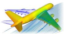 There are a lot of reasons for lack of progress in CFD codes, and here I will examine one particular issue. The reality is that there is a myriad of issues plaguing modern codes. I’ve written about issues with our modeling and its lack of suitability for tackling modern simulation questions. One of the major issues is the declaration that success won’t be reached until computers are far more powerful. This is also testimony to the lack of faith in innovation and creativity in research (risk aversion and fear of failure being key). As a result funding and focus for improving the fundamentals of CFD codes has dried up. It like the community has collectively thrown up it hands and said, “its not worth it!”
The riskiest thing we can do is just maintain the status quo.
― Bob Iger
 We have an overly focused research program toward utilizing the next generation of computing hardware. The major overarching issue is a general lack of risk taking in our research programs spanning from government funded pure research, through applied research programs and extending to industrially focused research. Without a tolerance for failure and hence a risk, the ability to make progress is utterly undermined. This more than anything explains why the codes are generally vehicles of status quo practice rather than dynamos of innovation.
Yesterday’s adaptations are today’s routines.
― Ronald A. Heifetz
If one travels back into the mid-1980’s there was a massive revolution in numerical methods in CFD codes. Methods that were introduced at that time remain at the core of CFD codes today. The reason was the development of new methods that were so unambiguously better than the previous alternatives that the change was a fait accompli. Codes produced results with the new methods that were impossible to achieve with previous methods. At that time a broad and important class of physical problems in fluid dynamics were suddenly open to successful simulation. Simulation results were more realistic and physically appealing and the artificial and unphysical results of the past were no longer a limitation.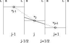
These methods were high-resolution methods such as flux corrected transport (FCT), high-order Godunov, total variation diminishing (TVD), and other formulations for solving hyperbolic conservation laws. These terms are in other words the convective or inertial terms in the governing equations transporting quantities through waves most typically through the bulk motion of the fluid. These new (at that time) methods produced results that when compared with preceding options were simply superior by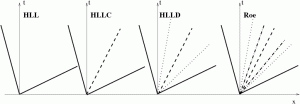 virtually any conceivable standard. In addition, the new methods were not either overly complex or expensive to use. The principles associated with their approach to solving the equations combined the best, most appealing aspects of previous methods in a novel fashion. They became the standard method almost overnight.
Novelty does not require intelligence, but ignorance, which is why the young excel in this branch.
― Anthony Marais
 This was accomplished because the methods were nonlinear even for linear equations meaning that the domain of dependence for the approximation is a function of the solution itself. Earlier methods were linear meaning that the approximation was the same without regard for the solution. Before the high-resolution methods you had two choices either a low-order method that would wash out the solution, or a high-order solution that would have unphysical solutions. Theoretically the low-order solution is superior in a sense because the solution could be guaranteed to be physical. This happened because the solution was found using a great deal of numerical or artificial viscosity. The solutions were effectively laminar (meaning viscously dominated) thus not having energetic structures that make fluid dynamics so exciting, useful and beautiful.
When your ideas shatter established thought, expect blowback.
― Tim Fargo
The new methods would use higher accuracy approximations as much as possible (or safe to do so), and only use the lower accuracy, dissipative method when absolutely necessary. Making these choices on the fly is the core of the magic of these methods. The new methods alleviated the bulk of this viscosity, but did not entirely remove it. This is good and important because some viscosity in the solution is essential to connect the results to the real world. Real world flows all have some amount of viscous dissipation. This fact is essential for success in computing shock waves where having dissipation allows the selection of the correct solution.
The status quo is never news, only challenges to it.
― Malorie Blackman
The dissipation is the essence of important phenomena such as turbulence as well. The viscous nature of things can be seen through a technique known as the method of modified equations. This method of numerical analysis derives the equations that the numerical method effectively solves. Because of numerical error when you solve an equation numerically, the solution more closely matches a more complex equation.
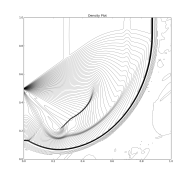 In the case of simple hyperbolic conservation laws that define the inertial part of fluid dynamics, the low order accuracy methods solve an equation with classical viscous terms that match those seen in reality although generally the magnitude of viscosity is much larger than the real world. Thus these methods produce laminar (syrupy) flows as a matter of course. This makes these methods unsuitable for simulating most conditions of interest to engineering and science. It also makes these methods very safe to use and virtually guarantee a physically reasonable (if inaccurate) solution.
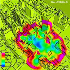 The new methods get rid of these large viscous terms and replace it with a smaller viscosity that depends on the structure of the solution. The results with the new methods are stunningly different and produce the sort of rich nonlinear structures found in nature (or something closely related). Suddenly codes produced solutions that matched reality far more closely. It was a night and day difference in method performance, once you tried the new methods there was no going back.
Negative results are just what I want. They’re just as valuable to me as positive results. I can never find the thing that does the job best until I find the ones that don’t.
― Thomas A. Edison
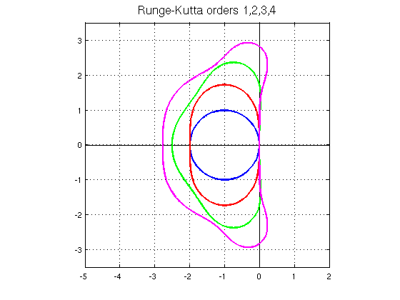
This is the crux of the issue with moving on to even more advanced methods, the quantum leap in performance to be had then simply won’t be repeated. The newer methods will not yield a change like the initial movement to high-resolution methods. The newer methods will be better and more accurate, but not Earth-shatteringly so. In today’s risk adverse world making a change for the sake of continual improvement is almost impossible to sell. The result is stagnation and lack of progress.
The problems don’t end there by a long shot. Because of the massive improvement in solutions to be had with the first generation of high resolution methods to a very large extent cost wasn’t an issue. With the next generation of methods, the improvements are far more modest and the cost of using them is an issue. So far, these methods are simply too expensive to displace the older methods.
The issues don’t even stop there. The new methods also tend to have relatively large errors compared to their cost. In addition the newer methods tend to be fragile and may not handle difficult situations robustly. The demands of maintaining formally high-order accuracy are quite expensive (time, space integration demands are costly whereas the first generation high resolution methods are simple and cheap). The result is that the newer approaches are methods that “do not pay their way.”
The balance of accuracy and cost has not been negotiated well. This whole dynamic is worth a good bit of discussion.
The key to this issue is the lack of capacity for high-order accuracy to be achieved in practical problems. To get high-order accuracy the solution needs to be smooth and differentiable. Real problems conspire against this sort of character at virtually every turn with singular structures both in the solution itself, not to mention geometry or physical properties. Real objects are rough and imperfect, which tends to breed more structure in solutions. Shock waves are the archetype of the problem that undermines high-order accuracy, but the problem hardly stops there.
The measure of intelligence is the ability to change.
― Albert Einstein
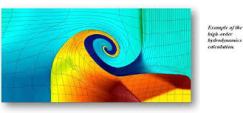 All of these factors conspire to produce in real problems, results only improve their accuracy at first-order (or worse), which means that double the mesh produces half the error. In other words, the accuracy is linearly proportional to the mesh spacing. This is a big deal as the second-order means that halving the mesh yields a four times reduction in error. Third-order would yield an eight times reduction. The reality is everything gives first-order accuracy or worse. The key for high-order working at all is that the high-order methods give a lower starting point for the error, which it sometimes does. The problem is that high-order methods are too expensive to justify the improvements they provide. The question is whether the benefits of practical accuracy can be achieved without incurring the costs typical for such methods.
Sometimes a clearly defined error is the only way to discover the truth
― Benjamin Wiker
The higher costs of the high-order methods are associated with a multitude of the characteristics of these methods. The basic steps associated with creating the high-order approximations use more data an d involve many more operations than existing methods. If this wasn’t bad enough these methods often require a multiple of evaluations to integrate their approximations using quadratures. In cases of time-dependent methods, these methods often require more steps and require smaller time steps than the standard methods. To make matters even worse these methods are often not applicable to complex geometries associated with real problems. If you add on relative fragility and small gains in practical accuracy, you get the state of affairs we see today.
Restlessness is discontent — and discontent is the first necessity of progress. Show me a thoroughly satisfied man — and I will show you a failure.
― Thomas A. Edison
Meanwhile the theoretical and mathematical communities will tie themselves to high formal order of accuracy even when the methods are inefficient. The very communities that we should depend on to break this log jam are not motivated to deal with the actual problem. We are left in a lurch where no progress is being made toward improving the work horse methods in our codes.
To improve is to change; to be perfect is to change often.
― Winston S. Churchill
 The cost part is almost a uniformly disappointing part of these methods most of which is dedicated to achieving formally high-order results. The irony is that the formal order of accuracy is immaterial to their practical and pragmatic utility. Almost no effort has been devoted to understanding how this cost accuracy dynamic can be negotiated. Without progress and understanding of these issues, the older methods, which now are standard will simply not move forward. Thus we had a great leap forward 25-30 years ago followed by stasis and stagnation.
Change almost never fails because it’s too early. It almost always fails because it’s too late.
― Seth Godin
Here are some “fun” research papers to read on these topics.
[Harten83] Harten, Ami. “High resolution schemes for hyperbolic conservation laws.”Journal of computational physics 49, no. 3 (1983): 357-393.
[HEOC87] Harten, Ami, Bjorn Engquist, Stanley Osher, and Sukumar R. Chakravarthy. “Uniformly high order accurate essentially non-oscillatory schemes, III.” Journal of computational physics 71, no. 2 (1987): 231-303.
| [HHL76] Harten, Amiram, James M. Hyman, Peter D. Lax, and Barbara Keyfitz. “On finite‐difference approximations and entropy conditions for shocks.”Communications on pure and applied mathematics 29, no. 3 (1976): 297-322. |
[Lax73] Lax, Peter D. Hyperbolic systems of conservation laws and the mathematical theory of shock waves. Vol. 11. SIAM, 1973.
[LW60] Lax, Peter, and Burton Wendroff. “Systems of conservation laws.”Communications on Pure and Applied mathematics 13, no. 2 (1960): 217-237.
[Boris71] Boris, Jay P., and David L. Book. “Flux-corrected transport. I. SHASTA, A fluid transport algorithm that works.” Journal of computational physics 11, no. 1 (1973): 38-69.
(Boris, Jay P. A Fluid Transport Algorithm that Works. No. NRL-MR-2357. NAVAL RESEARCH LAB WASHINGTON DC, 1971.)
[VanLeer73] van Leer, Bram. “Towards the ultimate conservative difference scheme I. The quest of monotonicity.” In Proceedings of the Third International Conference on Numerical Methods in Fluid Mechanics, pp. 163-168. Springer Berlin Heidelberg, 1973.
[Shu87] Shu, Chi-Wang. “TVB uniformly high-order schemes for conservation laws.”Mathematics of Computation 49, no. 179 (1987): 105-121.
[GLR07] Grinstein, Fernando F., Len G. Margolin, and William J. Rider, eds. Implicit large eddy simulation: computing turbulent fluid dynamics. Cambridge university press, 2007.
[RM05] Margolin, L. G., and W. J. Rider. “The design and construction of implicit LES models.” International journal for numerical methods in fluids 47, no. 10‐11 (2005): 1173-1179.
[MR02] Margolin, Len G., and William J. Rider. “A rationale for implicit turbulence modelling.” International Journal for Numerical Methods in Fluids 39, no. 9 (2002): 821-841.



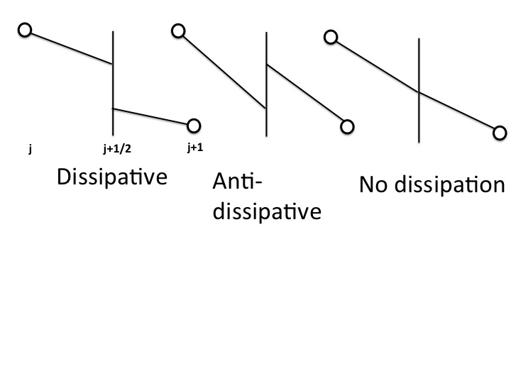 All of these techniques will utilize an important observation for methods of this type; one can swap edge-face values without impacting the accuracy of the method. Consider the reconstructed edge value


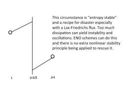 as “entropy stable”. The condition can be computed by checking whether the jump in edge values


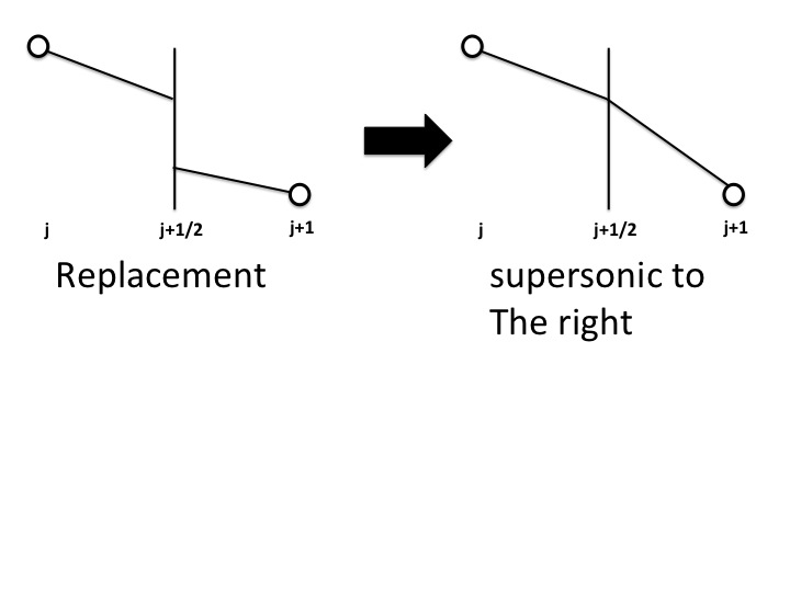 centered edge values, the fifth-order upwind to sixth-order centered, and so forth.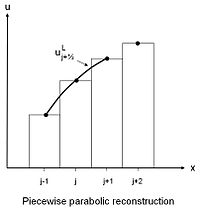
 where
where  , the limiter is implemented as
  ,
,  is the general limiter and
  . The limiter has a general form,
  . The “Standard” is the test that defines the nonlinear control of the solution while “Reconstruction Choice” is the feature being controlled. I will give some examples below. It is important to note that
  is the reconstruction that produces an upwind scheme that is the canonical linear monotonicity preserving (positive) method, but only first-order accurate. Higher order polynomials can be defined for higher accuracy, but without the limiter they are invariably oscillatory.
 where
where  is the lowest value of
  that will be tolerated for physical reasons. Next our reconstruction is interrogated
 ![\mbox{Reconstruction Choice} = u_j -\min\left[p\left(\theta\right)\right]](https://s0.wp.com/latex.php?latex=%5Cmbox%7BReconstruction+Choice%7D+%3D+u_j+-%5Cmin%5Cleft%5Bp%5Cleft%28%5Ctheta%5Cright%29%5Cright%5D&bg=ffffff&fg=000&s=0&c=20201002) .
. here
here  is the famous minimum modulus function that returns the smallest magnitude argument if the arguments have the same sign.
  where
where  is the “high-order” slope that you desire to use and control the stability of.
 ,
,  and everything else follows. The parts of the limiter are
  with
with  being the monotonicity preserving edge value,
  is the high-order edge values and
  is the WENO edge value. Next, the limiter is completed with
  . Part of the key idea is to use two complimentary nonlinear stability properties from monotonicity preservation and WENO to assure the stability of the method should the high-order method be chosen. In this case the high-order method is bounded by two nonlinearly stable approximation choices. I thought it actually worked pretty well.
 . In this case the specifics of the limiter are
  where
where  is the classical second derivative on the mesh and
  . The choice of method to define the denominator in the limiter is
  . The resulting limiter can either be applied to the edge values or equivalently to the reconstructing polynomial.

 with
with  being a constant. At its core is the imposition of reality on idealized math to describe reality, and provide a useful, utilitarian description of mathematically singular structures. This character is present in turbulence as well. Both have basically the same scaling law and deep philosophical implications.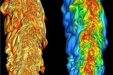










 wheelhouse (along with all the hijinks that the child movie viewers will enjoy).






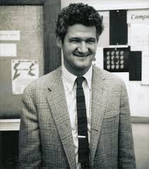
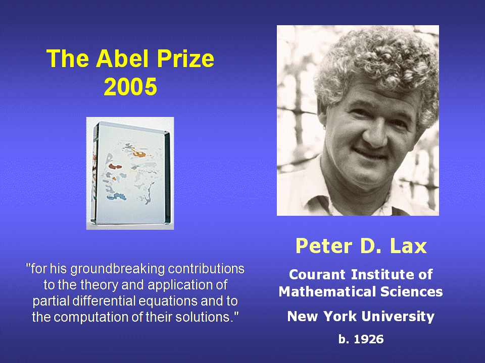
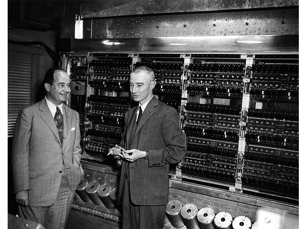
 The publisher is the American Mathematical Society (AMS) and the book is a wonderfully technical and personal account of the fascinating and influential life of Peter Lax. Hersh’s account goes far beyond the obvious public and professional impact of Lax into his personal life and family although these are colored greatly by the greatest events of the 20th Century. Lax also has a deep connection to three themes in my own life: scientific computing, hyperbolic conservation laws and Los Alamos. He was a contributing member of the Manhattan Project despite being a corporal in the US Army and only 18 years old! Los Alamos and John von Neumann in particular had an immense influence on his life’s work with the fingerprints of that influence all over his greatest professional achievements.